User:Kazkaskazkasako/Books/Mathematics

Mathematics

Fields of mathematics

Category:Fields of mathematics

Category:Game theory

List of important publications in mathematics: Algebra: Theory of equations, Abstract algebra: Group theory, Homological algebra. Algebraic geometry. Number theory. Analysis: Calculus, Functional analysis, Fourier analysis. Geometry: Differential geometry. Topology. Category theory. Set theory. Logic. Combinatorics: Graph theory. Computational complexity theory. Probability theory and statistics. Game theory. Fractals. Numerical analysis: Optimization. Early manuscripts. Textbooks. Popular writings.

Curry-Howard correspondence 1934, direct relationship between computer programs and mathematical proofs, functional programming languages: Haskell & co

Simple maths:

Indeterminate (variable)

Indeterminate form

Hardcore math: stats (the biggest lie) - Markovian chains, Bayesian probability and inference

Optimization, aka mathematical programming: Great Deluge algorithm, Hill climbing, Simulated annealing

Graph invariant (graph invariant): property of graphs that depends only on the abstract structure, not on graph representations such as particular labellings or drawings of the graph. Graph canonization (canonical form of a graph, canonical labeling of a graph, graph canonicalization).

Mathematical notation

Category:Mathematical notation

Category:Mathematical markup languages

Category:Numeral systems

Category:Positional numeral systems

Glossary of mathematical symbols (aka List of mathematical symbols): figure or a combination of figures that is used to represent a mathematical object, an action on mathematical objects, a relation between mathematical objects, or for structuring the other symbols that occur in a formula. As formulas are entirely constituted with symbols of various types, many symbols are needed for expressing all mathematics.

• Layout of this article: Normally, entries of a glossary are structured by topics and sorted alphabetically. This is not possible here, as there is no natural order on symbols, and many symbols are used in different parts of mathematics with different meanings, often completely unrelated. Most symbols have two printed versions. They can be displayed as Unicode characters, or in LaTeX format. With the Unicode version, using search engines and copy-pasting are easier. On the other hand, the LaTeX rendering is often much better (more aesthetic), and is generally considered a standard in mathematics. Therefore, in this article, the Unicode version of the symbols is used (when possible) for labelling their entry, and the LaTeX version is used in their description. So, for finding how to type a symbol in LaTeX, it suffices to look at the source of the article.
• Arithmetic operators
• Equality, equivalence and similarity
• Comparison
• Set theory
• Basic logic
• Blackboard bold
• Calculus
• Linear and multilinear algebra
• Advanced group theory
• Infinite numbers
• Brackets
  • Parentheses
  • Square brackets
  • Braces
  • Other brackets
• Symbols that do not belong to formulas
• Miscellaneous

Mathematical operators and symbols in Unicode: Unicode Standard encodes almost all standard characters used in mathematics. Unicode Technical Report #25 provides comprehensive information about the character repertoire, their properties, and guidelines for implementation. Mathematical operators and symbols are in multiple Unicode blocks. Some of these blocks are dedicated to, or primarily contain, mathematical characters while others are a mix of mathematical and non-mathematical characters. This article covers all Unicode characters with a derived property of "Math".

Nations based on the decimal separator in use. Full stop/Period (.); Comma (,); Both, official or common or apostrophe ('); Momayyez (٫)

Decimal separator (decimal mark, decimal marker, decimal sign; decimal point vs decimal comma): symbol used to separate the integer part from the fractional part of a number written in decimal form. Different countries officially designate different symbols for use as the separator. The choice of symbol also affects the choice of symbol for the thousands separator used in digit grouping. The 22nd General Conference on Weights and Measures declared in 2003 that "the symbol for the decimal marker shall be either the point on the line or the comma on the line". It further reaffirmed that "numbers may be divided in groups of three in order to facilitate reading; neither dots nor commas are ever inserted in the spaces between groups" (e.g. 1000000000).

Radix point: symbol used in numerical representations to separate the integer part of a number (to the left of the radix point) from its fractional part (to the right of the radix point). "Radix point" applies to all number bases. In base 10 notation, the radix point is more commonly called the decimal point, where the prefix deci- implies base 10. Similarly, the term "binary point" is used for base 2.

Basic Maths

Category:Constants

Category:Mathematical constants

Category:Mathematical objects

Mathematical constant: π, e, ...

Mathematical object: abstract object arising in philosophy of mathematics and mathematics. Commonly encountered mathematical objects include numbers, permutations, partitions, matrices, sets, functions, and relations. Geometry as a branch of mathematics has such objects as hexagons, points, lines, triangles, circles, spheres, polyhedra, topological spaces and manifolds. Another branch - Algebra, has groups, rings, fields, group-theoretic lattices, and order-theoretic lattices. Categories are simultaneously homes to mathematical objects and mathematical objects in their own right.

"Roots" of maths (sets of axioms) and deep philosophy

Axiom of choice ≡ Zorn's lemma? R&U

Homology (mathematics): original motivation for defining homology groups is the commonplace observation that one aspect of the shape of an object is its holes. But because a hole is "not there", it is not immediately obvious how to define a hole, or how to distinguish between different kinds of holes. Homology is a rigorous mathematical method for detecting and categorizing holes in a shape.

Homotopy group vs Topology:

Homotopy group carry information about the global structure.

Topology deals only with the local structure.

Function

Category:Analytic functions

Category:Functions and mappings

Category:Types of functions

Function (mathematics)

Function range: image f $\subseteq$ range f $\subseteq$ co-domain f, with one or the other containment being equality. Domain of a function→(codomain, (image))

Pigeonhole principle (aka: Dirichlet's box principle or Dirichlet's drawer principle; DE: Schubfachprinzip): if n items are put into m pigeonholes with n > m, then at least one pigeonhole must contain more than one item, formal definition: there does not exist an injective function on finite sets whose codomain is smaller than its domain.

Transcendental function: does not satisfy a polynomial equation whose coefficients are themselves polynomials, in contrast to an algebraic function, which does satisfy such an equation; function that "transcends" algebra in the sense that it cannot be expressed in terms of a finite sequence of the algebraic operations of addition, multiplication, and root extraction. E.g. exponential function, logarithm, and trigonometric functions.

Special functions

Category:Types of functions

Category:Special functions

Category:Elementary special functions

Category:Exponentials

mathematical operation, written as , involving two numbers, the base When n is a positive integer, exponentiation corresponds to repeated multiplication of the base: that is, bⁿ is the product of multiplying n bases:

Exponentiation: a mathematical operation, written as bⁿ, involving two numbers, the base b and the exponent or power n. When n is a positive integer, exponentiation corresponds to repeated multiplication of the base: that is, bⁿ is the product of multiplying n bases:

$b^{n}=\underbrace {b\times \dots \times b} _{n\,{\textrm {times}}}.$ The exponent is usually shown as a superscript to the right of the base. In that case, bⁿ is called "b raised to the n-th power", "b raised to the power of n", "the n-th power of b", "b to the n-th", or most briefly as "b to the n".

• Exponentiation is not commutative
• Exponentiation is not associative
• Without parentheses, the conventional order of operations in superscript notation is top-down (or right-associative), not bottom-up:

$b^{p^{q}}=b^{\left(p^{q}\right)},$ which is different from $\left(b^{p}\right)^{q}=b^{pq}.$

Logic (also philosophical sense), philosophy of mathematics

Category:Philosophy of mathematics

Category:Philosophy of mathematics literature

Category:Formalism (deductive)

Category:Large-scale mathematical formalization projects

Category:Logic

Category:Critical thinking

Category:Bias

Category:Cognitive biases

Category:Mathematical logic

Category:Large-scale mathematical formalization projects

Category:Recursion

Category:Fixed points (mathematics)

Category:Set theory

Category:Logical consequence

Category:Inference

Category:Statistical inference

{q.v.

• User:Kazkaskazkasako/Books/EECS#Programming languages
• User:Kazkaskazkasako/Books/All#Philosophy of logic

}

Outline of logic

Logical biconditional

Principia Mathematica (PM): three-volume work on the foundations of mathematics written by the philosophers Alfred North Whitehead and Bertrand Russell and published in 1910, 1912, and 1913. In 1925–27, it appeared in a second edition with an important Introduction to the Second Edition, an Appendix A that replaced ✸9 and all-new Appendix B and Appendix C. PM is not to be confused with Russell's 1903 The Principles of Mathematics. PM was originally conceived as a sequel volume to Russell's 1903 Principles, but as PM states, this became an unworkable suggestion for practical and philosophical reasons. PM, according to its introduction, had three aims: (1) to analyze to the greatest possible extent the ideas and methods of mathematical logic and to minimize the number of primitive notions and axioms, and inference rules; (2) to precisely express mathematical propositions in symbolic logic using the most convenient notation that precise expression allows; (3) to solve the paradoxes that plagued logic and set theory at the turn of the 20th-century, like Russell's paradox. This third aim motivated the adoption of the theory of types in PM. The theory of types adopts grammatical restrictions on formulas that rules out the unrestricted comprehension of classes, properties, and functions. It was in part thanks to the advances made in PM that, despite its defects, numerous advances in meta-logic were made, including Gödel's incompleteness theorems. For all that, PM is not widely used today: probably the foremost reason for this is its reputation for typographical complexity. Somewhat infamously, several hundred pages of PM precede the proof of the validity of the proposition 1+1=2.

Automated theorem proving

Computer-assisted proof

Interactive theorem proving: tools to develop formal proofs by man-machine collaboration. E.g. HOL (using MLs: Standard ML and Moscow ML; OCaml)

Standard ML: general-purpose, modular, functional programming language with compile-time type checking and type inference

FUTON bias (full text on the Net bias): bias in academic research, when researchers "concentrate on research published in journals that are available as full text on the internet, and ignore relevant studies that are not available in full text, thus introducing an element of bias into their search result"

No abstract available bias (NAA bias)

Hindsight bias (knew-it-all-along effect, creeping determinism): inclination, after an event has occurred, to see the event as having been predictable, despite there having been little or no objective basis for predicting it. Hindsight bias may cause memory distortion, where the recollection and reconstruction of content can lead to false theoretical outcomes. Such examples are present in the writings of historians describing outcomes of battles, physicians recalling clinical trials, and in judicial systems trying to attribute responsibility and predictability of accidents.

Survivorship bias: logical error of concentrating on the people or things that made it past some selection process and overlooking those that did not, typically because of their lack of visibility. This can lead to false conclusions in several different ways. It is a form of selection bias.

Bulletin of the Atomic Scientists: nonprofit organization concerning science and global security issues resulting from accelerating technological advances that have negative consequences for humanity.

Doomsday Clock: symbol which represents the likelihood of a man-made global catastrophe. Maintained since 1947 by the members of the Bulletin of the Atomic Scientists, The Clock is a metaphor for threats to humanity from unchecked scientific and technical advances. The Clock represents the hypothetical global catastrophe as "midnight" and the Bulletin's opinion on how close the world is to a global catastrophe as a number of "minutes" to midnight. The factors influencing the Clock are nuclear risk and climate change.

Inferences: steps in reasoning, moving from premises to logical consequences; etymologically, the word infer means to "carry forward". Inference is theoretically traditionally divided into deduction and induction, a distinction that in Europe dates at least to Aristotle (300s BCE). Deduction is inference deriving logical conclusions from premises known or assumed to be true, with the laws of valid inference being studied in logic. Induction is inference from particular premises to a universal conclusion. Human inference (i.e. how humans draw conclusions) is traditionally studied within the fields of logic, argumentation studies, and cognitive psychology; artificial intelligence researchers develop automated inference systems to emulate human inference. Statistical inference.

Set theory

Category:Set theory (Naive set theory; Axiomatic set theory; Internal set theory; Various versions of logic have associated sorts of sets (such as fuzzy sets in fuzzy logic))

Category:Basic concepts in set theory (foundational concepts of naive set theory)

Set theory: branch of mathematical logic that studies sets, which can be informally described as collections of objects. Although objects of any kind can be collected into a set, set theory, as a branch of mathematics, is mostly concerned with those that are relevant to mathematics as a whole. The modern study of set theory was initiated by the German mathematicians Richard Dedekind and Georg Cantor in the 1870s. In particular, Georg Cantor is commonly considered the founder of set theory. The non-formalized systems investigated during this early stage go under the name of naive set theory. After the discovery of paradoxes within naive set theory (such as Russell's paradox, Cantor's paradox and Burali-Forti paradox) various axiomatic systems were proposed in the early twentieth century, of which Zermelo–Fraenkel set theory (with or without the axiom of choice) is still the best-known and most studied.

Multiset (bag, mset): modification of the concept of a set that, unlike a set, allows for multiple instances for each of its elements. The number of instances given for each element is called the multiplicity of that element in the multiset. Multiset {a, a, a, b, b, b}, a and b both have multiplicity 3.

• Counting multisets: $\left(\!\!{n \choose k}\!\!\right)={n+k-1 \choose k}={\frac {(n+k-1)!}{k!\,(n-1)!}}={n(n+1)(n+2)\cdots (n+k-1) \over k!}$
  • Recurrence relation: $\left(\!\!{n \choose k}\!\!\right)=\left(\!\!{n \choose k-1}\!\!\right)+\left(\!\!{n-1 \choose k}\!\!\right)\quad {\mbox{for }}n,k>0$; with $\left(\!\!{n \choose 0}\!\!\right)=1,\quad n\in \mathbb {N} ,\quad {\mbox{and}}\quad \left(\!\!{0 \choose k}\!\!\right)=0,\quad k>0.$
  • Generating series
  • Generalization and connection to the negative binomial series

Tuple: finite ordered list (sequence) of elements. n-tuple is a sequence (or ordered list) of n elements, where n is a non-negative integer. There is only one 0-tuple, referred to as the empty tuple. An n-tuple is defined inductively using the construction of an ordered pair. Mathematicians usually write tuples by listing the elements within parentheses "( )" and separated by commas; for example, (2, 7, 4, 1, 7) denotes a 5-tuple. Relational databases may formally identify their rows (records) as tuples. Tuples also occur in relational algebra; when programming the semantic web with the Resource Description Framework (RDF); in linguistics; and in philosophy.

• Properties:
  • general rule for the identity of two n-tuples is $(a_{1},a_{2},\ldots ,a_{n})=(b_{1},b_{2},\ldots ,b_{n})$ if and only if $a_{1}=b_{1},{\text{ }}a_{2}=b_{2},{\text{ }}\ldots ,{\text{ }}a_{n}=b_{n}$
  1. tuple may contain multiple instances of the same element, so tuple $(1,2,2,3)\neq (1,2,3)$; but set $\{1,2,2,3\}=\{1,2,3\}$
  2. tuple elements are ordered: tuple $(1,2,3)\neq (3,2,1)$, but set $\{1,2,3\}=\{3,2,1\}$
  3. tuple has a finite number of elements, while a set or a multiset may have an infinite number of elements
• Definitions: Tuples as functions: Tuples as sets of ordered pairs; Tuples as nested ordered pairs; Tuples as nested sets
• n-tuples of m-sets
• Type theory

Combinatorics

Category:Combinatorics

Binomial coefficient (nCk ("n choose k")): positive integers that occur as coefficients in the binomial theorem. Commonly, a binomial coefficient is indexed by a pair of integers n ≥ k ≥ 0 and is written ${\tbinom {n}{k}}.$ It is the coefficient of the x^k (1 + x)ⁿ. It is the coefficient of the x^k term in the polynomial expansion of the binomial power (1 + x)ⁿ, and is given by the formula ${\binom {n}{k}}={\frac {n!}{k!(n-k)!}}.$ Arranging the numbers ${\tbinom {n}{0}},{\tbinom {n}{1}},\ldots ,{\tbinom {n}{n}}$ in successive rows for $n=0,1,2,\ldots$ gives a triangular array called Pascal's triangle, satisfying the recurrence relation (Recursive formula) ${\binom {n}{k}}={\binom {n-1}{k}}+{\binom {n-1}{k-1}}.$

• History and notation: Andreas von Ettingshausen introduced the notation ${\tbinom {n}{k}}$ in 1826. Alternative notations include C(n, k), _nC_k, ⁿC_k, C^k_n, Cⁿ_k, and C_n,k in all of which the C stands for combinations or choices.
• Definition and interpretations: $(x+y)^{n}=\sum _{k=0}^{n}{\binom {n}{k}}x^{n-k}y^{k}$
• Combinatorics and statistics:
  • ${\tbinom {n+k-1}{k}}$ ways to choose k elements from a set of n elements if repetitions are allowed
  • ${\tbinom {n+k}{k}}$ strings (EECS) containing k ones and n zeros
  • ${\tbinom {n+1}{k}}$ strings consisting of k ones and n zeros such that no two ones are adjacent
  • binomial distribution in statistics is ${\tbinom {n}{k}}p^{k}(1-p)^{n-k}\!.$
• Binomial coefficients as polynomials: Binomial coefficients as a basis for the space of polynomials; Integer-valued polynomials
• Identities involving binomial coefficients: Sums of the binomial coefficients: Multisections of sums, Partial sums; Identities with combinatorial proofs: Sum of coefficients row; Dixon's identity; Continuous identities; Congruences.
• Generating functions: Ordinary generating functions; Exponential generating function
• Divisibility properties
• Bounds and asymptotic formulas: Both n and k large; Sums of binomial coefficients; Generalized binomial coefficients
• Generalizations: Generalization to multinomials; Taylor series; Binomial coefficient with n = 1/2; Products of binomial coefficients; Partial fraction decomposition; Newton's binomial series; Multiset (rising) binomial coefficient: Generalization to negative integers n; Two real or complex valued arguments; Generalization to q-series; Generalization to infinite cardinals
• In programming languages

Probability and statistics ("biggest lie")

Category:Statistics

Category:Statistical theory

Category:Statistical inference

Category:Statistics profession and organizations

Category:Ethics and statistics

Category:Misuse of statistics

Glossary of probability and statistics

Timeline of probability and statistics

Template:Statistics

• Descriptive statistics:
  • Continuous data: Center (Mean, Median, Mode); Dispersion (Variance, Standard deviation, CV/RSD, Range, Interquartile Range (IQR)); Shape (Central limit theorem, Moments (Skewness, Kurtosis, L-moments))
  • Count data
  • Summary tables: Grouped data; Frequency distribution; Contingency table
  • Correlation and dependence: Scatter plot, ...
  • Statistical graphics
• Data collection:
  • Design of experiments (DOE): ...; Replication; Missing data
  • Survey methodology: Sampling (Stratified sampling, Cluster sampling); Standard error (SE, standard error of the mean (SEM)); Opinion poll; Questionnaire
  • Controlled experiments: Scientific control; Randomized experiments; Randomized controlled trial; Random assignment/placement; Blocking; Interaction; Factorial experiment
  • Adaptive Designs:
  • Observational study: Cross-sectional study; Cohort study; Natural experiment; Quasi-experiment
• Statistical inference:
  • Theory of statistics: Population; Statistic; Probability distribution; ...; Completeness; ...; Robustness
  • Frequentist inference: Point estimation; Interval estimation; Testing hypotheses; Parametric tests
  • Specific tests: Z-test (normal); Student's t-test; F-test. Goodness of fit: Chi-squared, ... ; Rank statistics: ...
  • Bayesian inference: Bayesian probability (prior, posterior), Credible interval, Bayes factor, Bayesian estimator (Maximum posterior estimator)
• Correlation and dependence | Regression analysis:
  • Correlation:
  • Regression analysis:
  • Linear regression:
  • Non-standard predictors:
  • Generalized linear model:
  • Partition of sums of squares: ANOVA, Analysis of covariance, multivariate ANOVA, Degrees of freedom
• Categorical variable | Multivariate statistics | Time series | Survival analysis:
  • Categorical variable: ..., Contingency table, ...
  • Multivariate statistics:
  • Time-series: General; Specific tests; Time domain (Autocorrelation (ACF), PACF; XCF; ARMA model; ARIMA model; ARCH; VAR); Frequency domain (Spectral density estimation, Fourier analysis, Wavelet, Whittle likelihood) {q.v. User:Kazkaskazkasako/Books/EECS#Signal processing, image processing}
  • Survival analysis: Survival function (...); Hazard function | Failure rate (...); Test (Log-rank test)
• List of fields of application of statistics:
  • Biostatistics: Bioinformatics; Clinical trials / studies; Epidemiology; Medical statistics
  • Engineering statistics: ...
  • Social statistics: Actuarial science; Census; Crime statistics; Demography; Econometrics; ...; Population statistics; ...
  • Spatial statistics: Cartography; Environmental statistics; GIS; Geostatistics; Kriging

List of statistics articles

List of important publications in statistics: Probability. Mathematical statistics. Bayesian statistics. Multivariate analysis. Time series. Applied statistics. Statistical learning theory. Variance component estimation. Survival analysis. Meta analysis. Experimental design.

Statistic (sample statistic): any quantity computed from values in a sample that is used for a statistical purpose. Statistical purposes include estimating a population parameter, describing a sample, or evaluating a hypothesis. When a statistic is used to estimate a population parameter, the statistic is called an estimator. A population parameter is any characteristic of a population under study, but when it is not feasible to directly measure the value of a population parameter, statistical methods are used to infer the likely value of the parameter on the basis of a statistic computed from a sample taken from the population. Note that a single statistic can be used for multiple purposes – for example the sample mean can be used to estimate the population mean, to describe a sample data set, or to test a hypothesis.

Variance: expectation of the squared deviation of a random variable from its mean, and it informally measures how far a set of (random) numbers are spread out from their mean. The variance is the square of the standard deviation, the second central moment of a distribution, and the covariance of the random variable with itself, often represented by σ², or $\operatorname {Var} (X)$.

Standard deviation (SD, σ): measure that is used to quantify the amount of variation or dispersion of a set of data values. A low standard deviation indicates that the data points tend to be close to the mean (also called the expected value) of the set, while a high standard deviation indicates that the data points are spread out over a wider range of values. The standard deviation of a population or sample and the standard error of a statistic (e.g., of the sample mean) are quite different, but related. The sample mean's standard error is the standard deviation of the set of means that would be found by drawing an infinite number of repeated samples from the population and computing a mean for each sample.

Standard error (SE): of a statistic (usually an estimate of a parameter) is the standard deviation of its sampling distribution or an estimate of that standard deviation. If the statistic is the sample mean, it is called the standard error of the mean (SEM). The sampling distribution of a population mean is generated by repeated sampling and recording of the means obtained. This forms a distribution of different means, and this distribution has its own mean and variance. Mathematically, the variance of the sampling distribution obtained is equal to the variance of the population divided by the sample size. This is because as the sample size increases, sample means cluster more closely around the population mean.

• Population: ${\sigma }_{\bar {x}}\ ={\frac {\sigma }{\sqrt {n}}}$, σ is SD of the population, n is the size (number of observations) of the sample.
• Estimate: ${\sigma }_{\bar {x}}\ \approx {\frac {s}{\sqrt {n}}}$, s is the sample standard deviation (i.e., the sample-based estimate of the standard deviation of the population), n is the size (number of observations) of the sample.
• Student approximation when σ value is unknown
• Assumptions and usage: Confidence interval

Law of large numbers (LLN): theorem that describes the result of performing the same experiment a large number of times. The average of the results obtained from a large number of trials should be close to the expected value, and will tend to become closer as more trials are performed.

Regression toward the mean: is it related to LLN just expressed in another, more linguistic less mathematical way?

King effect: phenomenon where the top one or two members of a ranked set show up as outliers (unexpectedly large because they do not conform to the statistical distribution or rank-distribution which the remainder of the set obeys).

Anscombe's quartet: second graph (top right) is not distributed normally; third graph (bottom left), the distribution is linear, but should have a robust regression; fourth graph (bottom right) shows an example when one high-leverage point is enough to produce a high correlation coefficient, even though the other data points do not indicate any relationship between the variables.

Anscombe's quartet: comprises four data sets that have nearly identical simple descriptive statistics, yet have very different distributions and appear very different when graphed. Each dataset consists of eleven (x,y) points. They were constructed in 1973 by the statistician Francis Anscombe to demonstrate both the importance of graphing data before analyzing it and the effect of outliers and other influential observations on statistical properties. He described the article as being intended to counter the impression among statisticians that "numerical calculations are exact, but graphs are rough."

Probability theory

Independence (probability theory): fundamental notion in probability theory, as in statistics and the theory of stochastic processes. Two events are independent, statistically independent, or stochastically independent if the occurrence of one does not affect the probability of occurrence of the other (equivalently, does not affect the odds). Similarly, two random variables are independent if the realization of one does not affect the probability distribution of the other.

• Cumulant: alternative to moments
• Standardized moment & central moment: second moment is variance, third standardized moment is skewness (measure of asymmetry of the probability distribution), fourth std. moment is kurtosis (measure of "peakedness" of the probability distribution)

Statistical distributions, probability distributions, statistical tests

Category:Exponential family distributions

Category:Normal distribution

Category:Probability distributions

Category:Continuous distributions

Probability distribution: mathematical function that gives the probabilities of occurrence of different possible outcomes for an experiment. It is a mathematical description of a random phenomenon in terms of its sample space and the probabilities of events (subsets of the sample space). Terminology:

• Functions for discrete variables:
  • Probability function
  • Probability mass function (pmf)
  • Frequency distribution
  • Relative frequency distribution
  • Discrete probability distribution function
  • Cumulative distribution function
  • Categorical distribution
• Functions for continuous variables:
  • Probability density function (pdf)
  • Continuous probability distribution function
  • Cumulative distribution function (cdf)
  • Quantile function
• Basic terms:
  • Mode
  • Support: set of values that can be assumed with non-zero probability by the random variable.
  • Tail
  • Head
  • Expected value or mean
  • Media
  • Variance
  • Standard deviation
  • Quantile
  • Symmetry
  • Skewness: measure of the extent to which a pmf or pdf "leans" to one side of its mean. The third standardized moment of the distribution.
  • Kurtosis: measure of the "fatness" of the tails of a pmf or pdf. The fourth standardized moment of the distribution.

Normalization (statistics): may refer to more sophisticated adjustments where the intention is to bring the entire probability distributions of adjusted values into alignment. In the case of normalization of scores in educational assessment, there may be an intention to align distributions to a normal distribution. In another usage in statistics, normalization refers to the creation of shifted and scaled versions of statistics, where the intention is that these normalized values allow the comparison of corresponding normalized values for different datasets in a way that eliminates the effects of certain gross influences, as in an anomaly time series. Some types of normalization involve only a rescaling, to arrive at values relative to some size variable. In terms of levels of measurement, such ratios only make sense for ratio measurements (where ratios of measurements are meaningful), not interval measurements (where only distances are meaningful, but not ratios). Examples of normalizations:

• ${\frac {X-\mu }{\sigma }}$ Standard score; Z-score
• ${\frac {{\widehat {\beta }}-\beta _{0}}{\operatorname {s.e.} ({\widehat {\beta }})}}$ Student's t-statistic, ${\operatorname {s.e.} }$ standard error

List of probability distributions

Dirac delta function (δ function): generalized function or distribution introduced by physicist Paul Dirac. It is used to model the density of an idealized point mass or point charge as a function equal to zero everywhere except for zero and whose integral over the entire real line is equal to one. As there is no function that has these properties, the computations made by theoretical physicists appeared to mathematicians as nonsense until the introduction of distributions by Laurent Schwartz to formalize and validate the computations. As a distribution, the Dirac delta function is a linear functional that maps every function to its value at zero. In engineering and signal processing, the delta function, also known as the unit impulse symbol, may be regarded through its Laplace transform, as coming from the boundary values of a complex analytic function of a complex variable.

Normal distribution (${\mathcal {N}}(\mu ,\sigma ^{2})$; Gaussian distribution, Laplace–Gaus distribution): type of continuous probability distribution for a real-valued random variable. The parameter μ is the mean or expectation of the distribution (and also its median and mode), while the parameter σ is its standard deviation. The variance of the distribution is σ². A random variable with a Gaussian distribution is said to be normally distributed, and is called a normal deviate. A normal distribution is sometimes informally called a bell curve. Normal distributions are important in statistics and are often used in the natural and social sciences to represent real-valued random variables whose distributions are not known. Their importance is partly due to the central limit theorem. It states that, under some conditions, the average of many samples (observations) of a random variable with finite mean and variance is itself a random variable—whose distribution converges to a normal distribution as the number of samples increases. Therefore, physical quantities that are expected to be the sum of many independent processes, such as measurement errors, often have distributions that are nearly normal. $f(x)={\frac {1}{\sigma {\sqrt {2\pi }}}}e^{-{\frac {1}{2}}\left({\frac {x-\mu }{\sigma }}\right)^{2}}$

Standard score: number of standard deviations by which the value of a raw score (i.e., an observed value or data point) is above or below the mean value of what is being observed or measured. Raw scores above the mean have positive standard scores, while those below the mean have negative standard scores. This process of converting a raw score into a standard score is called standardizing or normalizing. Standard scores are most commonly called z-scores; the two terms may be used interchangeably, as they are in this article. Other terms include z-values, normal scores, and standardized variables.

Standard normal table (unit normal table, Z table): mathematical table for the values of Φ, which are the values of the cumulative distribution function of the normal distribution. It is used to find the probability that a statistic is observed below, above, or between values on the standard normal distribution, and by extension, any normal distribution. Since probability tables cannot be printed for every normal distribution, as there are an infinite variety of normal distributions, it is common practice to convert a normal to a standard normal and then use the standard normal table to find probabilities. Conversion: $Z={\frac {X-\mu }{\sigma }}$; $Z={\frac {{\overline {X}}-\mu }{\sigma /{\sqrt {n}}}}$.

Student's t-distribution: any member of a family of continuous probability distributions that arise when estimating the mean of a normally-distributed population in situations where the sample size is small and the population's standard deviation is unknown. It was developed by English statistician William Sealy Gosset under the pseudonym "Student". ${\frac {{\bar {X}}-\mu }{S/{\sqrt {n}}}}$ - Student's t-distribution with $n-1$ degrees of freedom; (Bessel-corrected) sample variance: $S^{2}={\frac {1}{n-1}}\sum _{i=1}^{n}(X_{i}-{\bar {X}})^{2}$.

t-statistic: ratio of the departure of the estimated value of a parameter from its hypothesized value to its standard error. It is used in hypothesis testing via Student's t-test. The t-statistic is used in a t-test to determine if you should support or reject the null hypothesis. It is very similar to the Z-score but with the difference that t-statistic is used when the sample size is small or the population standard deviation is unknown. For example, the t-statistic is used in estimating the population mean from a sampling distribution of sample means if the population standard deviation is unknown. It is also used along with p-value when running hypothesis tests where the p-value tells us what the odds are of the results to have happened.

Chi-square distribution ($\chi ^{2}(k)\;$ or $\chi _{k}^{2}\!$; chi-squared): with k degrees of freedom is the distribution of a sum of the squares of k independent standard normal random variables. The chi-square distribution is a special case of the gamma distribution and is one of the most widely used probability distributions in inferential statistics, notably in hypothesis testing and in construction of confidence intervals. The chi-square distribution is used in the common chi-square tests for goodness of fit of an observed distribution to a theoretical one, the independence of two criteria of classification of qualitative data, and in confidence interval estimation for a population standard deviation of a normal distribution from a sample standard deviation.

Chi-squared test (χ² test): statistical hypothesis test that is valid to perform when the test statistic is chi-squared distributed under the null hypothesis, specifically Pearson's chi-squared test and variants thereof. Pearson's chi-squared test is used to determine whether there is a statistically significant difference between the expected frequencies and the observed frequencies in one or more categories of a contingency table.

F-distribution (Fisher–Snedecor distribution): continuous probability distribution that arises frequently as the null distribution of a test statistic, most notably in ANOVA, e.g., F-test.

Logistic distribution: continuous probability distribution. Its cumulative distribution function is the logistic function, which appears in logistic regression and feedforward neural networks. It resembles the normal distribution in shape but has heavier tails (higher kurtosis).

Loss function {q.v. User:Kazkaskazkasako/Books/EECS#Artificial intelligence (AI), machine learning (ML)}

Unbiased estimation of standard deviation

Statistical inference

Category:Statistical inference

Category:Estimation theory

Category:Errors and residuals

Category:Statistical hypothesis testing

{q.v.

• User:Kazkaskazkasako/Books/EECS#Data science, information science

}

Statistical inference: process of using data analysis (@data science) to infer properties of an underlying distribution of probability. Inferential statistical analysis infers properties of a population, for example by testing hypotheses and deriving estimates. It is assumed that the observed data set is sampled from a larger population.

Confidence interval (CI): type of estimate computed from the statistics of the observed data. This proposes a range of plausible values for an unknown parameter (for example, the mean). The interval has an associated confidence level that the true parameter is in the proposed range. The confidence level is chosen by the investigator. For a given estimation in a given sample, using a higher confidence level generates a wider (i.e., less precise) confidence interval. In general terms, a confidence interval for an unknown parameter is based on sampling the distribution of a corresponding estimator. Most commonly, a 95% confidence level is used.

• Basic steps: assume that the samples are drawn from a normal distribution; sample mean, ${\bar {x}}$; whether the population standard deviation is known, $\sigma$, or is unknown and is estimated by the sample standard deviation $s$.
  • If the population standard deviation is known then $z^{*}=\Phi ^{-1}\left(1-{\frac {\alpha }{2}}\right)=-\Phi ^{-1}\left({\frac {\alpha }{2}}\right)$, where $C=100(1-\alpha )\%$ is the confidence level and $\Phi$ is CDF of standard normal distribution, used as the critical value. This value is only dependent on the confidence level for the test. $\left({\bar {x}}-z^{*}{\sigma \over {\sqrt {n}}},{\bar {x}}+z^{*}{\sigma \over {\sqrt {n}}}\right)$
  • If the population standard deviation is unknown then the Student's t distribution is used as the critical value. This value is dependent on the confidence level (C) for the test and degrees of freedom ($=n-1$). $\left({\bar {x}}-t^{*}{s \over {\sqrt {n}}},{\bar {x}}+t^{*}{s \over {\sqrt {n}}}\right)$
• Significance of t-tables and z-tables: t-values are used when the sample size is below 30 and the standard deviation is unknown.

Margin of error: statistic expressing the amount of random sampling error in the results of a survey. The larger the margin of error, the less confidence one should have that a poll result would reflect the result of a survey of the entire population. The margin of error will be positive whenever a population is incompletely sampled and the outcome measure has positive variance, which is to say, the measure varies. For a simple yes/no poll $P$ as a sample of $n$ respondents drawn from a population $N{\text{, }}(n<<N)$ reporting the percentage $p$ of yes responses: $MOE_{\gamma }=z_{\gamma }\times {\sqrt {\frac {\sigma ^{2}}{n}}}$ (@SEM).

Statistical significance

p-value (AMA (USA Medical Association): P value; APA (USA Psychological Association): p value; ASA (USA Statistical Association): p-value): in null hypothesis significance testing is probability of obtaining test results at least as extreme as the results actually observed, under the assumption that the null hypothesis is correct. A very small p-value means that such an extreme observed outcome would be very unlikely under the null hypothesis. Reporting p-values of statistical tests is common practice in academic publications of many quantitative fields. Since the precise meaning of p-value is hard to grasp, misuse is widespread and has been a major topic in metascience. General definition and interpretation: consider an observed test-statistic $t$ from unknown distribution $T$. Then the p-value $p$ is what the prior probability would be of observing a test-statistic value at least as "extreme" as $t$ if null hypothesis $H$ were true. That is:

• $p=\Pr(T\geq t|H)$ for a one-sided right-tail test,
• $p=\Pr(T\leq t|H)$ for a one-sided left-tail test,
• $p=\Pr(abs(T)\geq abs(t)|H)$ for a two-sided test,

If the p-value is very small, then the statistical significance is thought to be very large: under the hypothesis under consideration, something very unlikely has occurred.

Misuse of p-values

Statistical hypothesis testing: t-test, z-test, chi-square, F test

Type I and type II errors: in statistical hypothesis testing, a type I error is the rejection of a true null hypothesis (also known as a "false positive" finding or conclusion; example: "an innocent person is convicted"), while a type II error is the non-rejection of a false null hypothesis (also known as a "false negative" finding or conclusion; example: "a guilty person is not convicted"). Much of statistical theory revolves around the minimization of one or both of these errors, though the complete elimination of either is a statistical impossibility for non-deterministic algorithms.

• Statistical background: H₀ - null hypothesis, H₁ - alternative hypothesis. Conceptually similar to the judgement in a court trial. The null hypothesis corresponds to the position of defendant: just as he is presumed to be innocent until proven guilty, so is the null hypothesis presumed to be true until the data provide convincing evidence against it. The alternative hypothesis corresponds to the position against the defendant.
• Table of error types

Table of error types		Null hypothesis (H0) is
		True	False
Decision about null hypothesis (H0)	Don't reject	Correct inference (true negative) (probability = 1−α)	Type II error (false negative) (probability = β)
	Reject	Type I error (false positive) (probability = α)	Correct inference (true positive) (probability = 1−β)

• • type I error rate or significance level is denoted by the Greek letter α (alpha) and is also called the alpha level.
  • rate of the type II error is denoted by the Greek letter β (beta) and related to the power of a test, which equals 1−β.

Power of a test of a binary hypothesis test is the probability that the test correctly rejects the null hypothesis ($H_{0}$) when a specific alternative hypothesis ($H_{1}$) is true. It is commonly denoted by $1-\beta$, and represents the chances of a "true positive" detection conditional on the actual existence of an effect to detect. Statistical power ranges from 0 to 1, and as the power of a test increases, the probability $\beta$ of making a type II error by wrongly failing to reject the null hypothesis decreases.

Errors and residuals: two closely related and easily confused measures of the deviation of an observed value of an element of a statistical sample from its "true value" (not necessarily observable). The error of an observation is the deviation of the observed value from the true value of a quantity of interest (for example, a population mean). The residual is the difference between the observed value and the estimated value of the quantity of interest (for example, a sample mean). The distinction is most important in regression analysis, where the concepts are sometimes called the regression errors and regression residuals and where they lead to the concept of studentized residuals. In econometrics, "errors" are also called disturbances.

Bayesian inference

Category:Statistical inference

Category:Bayesian inference

Category:Statistical forecasting

Category:Logic and statistics

Category:Conditional probability

Conditional probability: measure of the probability of an event occurring, given that another event (by assumption, presumption, assertion or evidence) has already occurred. If the event of interest is A and the event B is known or assumed to have occurred, "the conditional probability of A given B", or "the probability of A under the condition B", is usually written as P(A|B), or sometimes P_B(A) or P(A/B).

Bayesian inference:

$P(H|E)={\frac {P(E|H)\;P(H)}{P(E)}}$, where

• $H$ represents a specific hypothesis, which may or may not be some null hypothesis.
• $P(H)$ is called the prior probability of $H$ that was inferred before new evidence, $E$, became available.
• $P(E|H)$ is called the conditional probability of seeing the evidence $E$ if the hypothesis $H$ happens to be true. It is also called a likelihood function when it is considered as a function of $H$ for fixed $E$.
• $P(E)$ is called the marginal probability of $E$: the a priori probability of witnessing the new evidence $E$ under all possible hypotheses. It can be calculated as the sum of the product of all probabilities of any complete set of mutually exclusive hypotheses and corresponding conditional probabilities:

$P(E)=\sum P(E|H_{i})P(H_{i})$.

• $P(H|E)$ is called the posterior probability of $H$ given $E$.

Markov chain & Random walk

Stochastic matrix

Statistical models; regression analysis

Category:Statistical models

Category:Regression models

Category:Categorical regression models

Category:Econometric modeling

Category:Single-equation methods (econometrics)

Category:Categorical regression models

Category:Regression analysis

Category:Regression models

Category:Statistical classification

Category:Logistic regression

Category:Statistical data types

Category:Statistical classification

Category:Logistic regression

Regression analysis: set of statistical processes for estimating the relationships between a dependent variable (often called the 'outcome' or 'response' variable, or a 'label' in machine learning parlance) and one or more independent variables (often called 'predictors', 'covariates', 'explanatory variables' or 'features'). The most common form of regression analysis is linear regression, in which one finds the line (or a more complex linear combination) that most closely fits the data according to a specific mathematical criterion. First, regression analysis is widely used for prediction and forecasting, where its use has substantial overlap with the field of machine learning. Second, in some situations regression analysis can be used to infer causal relationships between the independent and dependent variables. Importantly, regressions by themselves only reveal relationships between a dependent variable and a collection of independent variables in a fixed dataset. To use regressions for prediction or to infer causal relationships, respectively, a researcher must carefully justify why existing relationships have predictive power for a new context or why a relationship between two variables has a causal interpretation. The latter is especially important when researchers hope to estimate causal relationships using observational data.

Logistic regression (logit model): statistical model that models the probability of an event taking place by having the log-odds for the event be a linear combination of one or more independent variables. In regression analysis, logistic regression (or logit regression) is estimating the parameters of a logistic model (the coefficients in the linear combination). Formally, in binary logistic regression there is a single binary dependent variable, coded by an indicator variable, where the two values are labeled "0" and "1", while the independent variables can each be a binary variable (two classes, coded by an indicator variable) or a continuous variable (any real value). The corresponding probability of the value labeled "1" can vary between 0 (certainly the value "0") and 1 (certainly the value "1"), hence the labeling; the function that converts log-odds to probability is the logistic function, hence the name. The unit of measurement for the log-odds scale is called a logit, from logistic unit, hence the alternative names.

Lasso (statistics) (least absolute shrinkage and selection operator; Lasso or LASSO): regression analysis method that performs both variable selection and regularization in order to enhance the prediction accuracy and interpretability of the resulting statistical model. It was originally introduced in geophysics, and later by Robert Tibshirani, who coined the term. Lasso was originally formulated for linear regression models.

Homoscedasticity and heteroscedasticity: in statistics, a sequence (or a vector) of random variables is homoscedastic (/ˌhoʊmoʊskəˈdæstɪk/) if all its random variables have the same finite variance; this is also known as homogeneity of variance. The complementary notion is called heteroscedasticity, also known as heterogeneity of variance. Assuming a variable is homoscedastic when in reality it is heteroscedastic (/ˌhɛtəroʊskəˈdæstɪk/) results in unbiased but inefficient point estimates and in biased estimates of standard errors, and may result in overestimating the goodness of fit as measured by the Pearson coefficient.

Curve fitting: Linear regression

Category:Curve fitting

Linear regression: linear approach for modelling the relationship between a scalar response and one or more explanatory variables (also known as dependent and independent variables). The case of one explanatory variable is called simple linear regression; for more than one, the process is called multiple linear regression. This term is distinct from multivariate linear regression, where multiple correlated dependent variables are predicted, rather than a single scalar variable. Assumptions: Weak exogeneity; Linearity; Constant variance (a.k.a. homoscedasticity): plot of the absolute or squared residuals versus the predicted values (or each predictor) can also be examined for a trend or curvature; Independence of errors; Lack of perfect multicollinearity in the predictors.

Model selection

Category:Statistical models

Category:Model selection

Category:Statistical inference

Category:Model selection

{q.v. User:Kazkaskazkasako/Books/EECS#Artificial intelligence (AI), machine learning (ML)}

Model selection: task of selecting a statistical model from a set of candidate models, given data. In the simplest cases, a pre-existing set of data is considered. However, the task can also involve the design of experiments such that the data collected is well-suited to the problem of model selection. Given candidate models of similar predictive or explanatory power, the simplest model is most likely to be the best choice (Occam's razor).

Cross-validation (statistics): any of various similar model validation techniques for assessing how the results of a statistical analysis will generalize to an independent data set. Cross-validation is a resampling method that uses different portions of the data to test and train a model on different iterations. One round of cross-validation involves partitioning a sample of data into complementary subsets, performing the analysis on one subset (called the training set), and validating the analysis on the other subset (called the validation set or testing set). To reduce variability, in most methods multiple rounds of cross-validation are performed using different partitions, and the validation results are combined (e.g. averaged) over the rounds to give an estimate of the model's predictive performance.

Time series

Category:Statistical forecasting

Category:Time series

Time series: a series of data points indexed (or listed or graphed) in time order. Most commonly, a time series is a sequence taken at successive equally spaced points in time. Thus it is a sequence of discrete-time data. Time series are very frequently plotted via run charts (a temporal line chart). Time series are used in statistics, signal processing, pattern recognition, econometrics, mathematical finance, weather forecasting, earthquake prediction, electroencephalography, control engineering, astronomy, communications engineering, and largely in any domain of applied science and engineering which involves temporal measurements. Time series analysis comprises methods for analyzing time series data in order to extract meaningful statistics and other characteristics of the data. Time series forecasting is the use of a model to predict future values based on previously observed values. While regression analysis is often employed in such a way as to test relationships between one more different time series, this type of analysis is not usually called "time series analysis", which refers in particular to relationships between different points in time within a single series. A stochastic model for a time series will generally reflect the fact that observations close together in time will be more closely related than observations further apart. In addition, time series models will often make use of the natural one-way ordering of time so that values for a given period will be expressed as deriving in some way from past values, rather than from future values (see time reversibility).

Multivariate statistics

Category:Multivariate statistics

Category:Analysis of variance (ANOVA)

Category:Dimension reduction

Category:Independence (probability theory)

Category:Regression analysis {q.v. #Statistical models; regression analysis}

Confounding (confounding variable, confounding factor, extraneous determinant, lurking variable): in statistics a confounder is a variable that influences both the dependent variable and independent variable, causing a spurious association. Confounding is a causal concept, and as such, cannot be described in terms of correlations or associations.

Spurious relationship (spurious correlation): mathematical relationship in which two or more events or variables are associated but not causally related, due to either coincidence or the presence of a certain third, unseen factor. Hypothesis testing. Detecting spurious relationships: Experiments; Non-experimental statistical analyses.

Explained variation: measures the proportion to which a mathematical model accounts for the variation (dispersion) of a given data set. The complementary part of the total variation is called unexplained or residual variation.

Statistical methods

Category:Statistics

Category:Statistical methods

Category:Statistical analysis

Category:Descriptive statistics

Category:Contingency table

Category:Statistical ratios

Contingency table (cross tabulation or crosstab): type of table in a matrix format that displays the (multivariate) frequency distribution of the variables; provide a basic picture of the interrelation between two variables and can help find interactions between them. A pivot table is a way to create contingency tables using spreadsheet software. Measures of association: Odds ratio, Phi coefficient, Cramér's V and the contingency coefficient C; Tetrachoric correlation coefficient; Lambda coefficient; Uncertainty coefficient; Others.

F-score (F-measure): measure of a test's accuracy. It is calculated from the precision and recall of the test, where the precision is the number of true positive results divided by the number of all positive results, including those not identified correctly, and the recall is the number of true positive results divided by the number of all samples that should have been identified as positive. Precision is also known as positive predictive value, and recall is also known as sensitivity in diagnostic binary classification:

$F_{1}={\frac {2}{\mathrm {recall^{-1}} +\mathrm {precision^{-1}} }}=2\cdot {\frac {\mathrm {precision} \cdot \mathrm {recall} }{\mathrm {precision} +\mathrm {recall} }}={\frac {\mathrm {tp} }{\mathrm {tp} +{\frac {1}{2}}(\mathrm {fp} +\mathrm {fn} )}}$.

Game, investment, gambling theory

Category:Fields of mathematics

Category:Game theory

Template:Game theory

philosophies of human interaction

Win-win game - people can seek mutual benefit in all human interactions. Principle-based behavior.

Win/Lose - The competitive paradigm: if I win, you lose. The leadership style is authoritarian. In relationships, if both people aren't winning, both are losing.

Lose/Win - The "Doormat" paradigm. The individual seeks strength from popularity based on acceptance. The leadership style is permissiveness. Living this paradigm can result in psychosomatic illness from repressed resentment.

No-win situation (Lose/Lose) - When people become obsessed with making the other person lose, even at their own expense. This is the philosophy of adversarial conflict, war, or of highly dependent persons. (If nobody wins, being a loser isn't so bad.)

Win - Focusing solely on getting what one wants, regardless of the needs of others.

Win/Win or No Deal - If we can't find a mutually beneficial solution, we agree to disagree agreeably - no deal. This approach is most realistic at the beginning of a business relationship or enterprise. In a continuing relationship, it's no longer an option.

Gambling and information theory

People: Claude Shannon & Edward O. Thorp (1960s, wearable computer in casino at rullette); John Larry Kelly, Jr.; Eudaemons (1970s, computer at rullette)

Kelly criterion (Kelly: strategy, formula, or bet): formula used to determine the optimal size of a series of bets. In most gambling scenarios, and some investing scenarios under some simplifying assumptions, the Kelly strategy will do better than any essentially different strategy in the long run.

Advantage gambling

Card counting: MIT Blackjack Team

Shuffling machine

Escalation of commitment: human behavior pattern in which an individual or group—when faced with increasingly negative outcomes from some decision, action, or investment—continues the same behavior rather than alter course. They maintain actions that are irrational, but align with previous decisions and actions. Economists and behavioral scientists use a related term, sunk cost fallacy, to describe the justification of increased investment of money, time, lives, etc. in a decision, based on the cumulative prior investment ("sunk costs"); despite new evidence suggesting that the cost, beginning immediately, of continuing the decision outweighs the expected benefit. In the context of military conflicts, sunk costs in terms of money spent and lives lost are often used to justify continued involvement.

Paradoxes

Sorites paradox (paradox of the heap; σωρείτης → sōreitēs → "heaped up"): "consider a heap of sand, from which grains are individually removed. Is it still a heap when only one grain remains? If not, when did it change from a heap to a non-heap?" The whole heap is digital, made of objects, as per this deduction the whole world and Universe are digital (?), therefore it's a huge simulation (?).

Coastline paradox: counterintuitive observation that the coastline of a landmass does not have a well-defined length. This results from the fractal-like properties of coastlines.

This goes even deeper: surface area as a projected area at the sea level is defined, whereas the surface area of the hills, mountains etc is not defined (even water reservoirs (lakes, seas) have ripples!). Because of our 3D world, is it possible to have a 3D volume which is so fractal, that the volume could not be measured? Surface-to-volume ratio is meaningless in 3D world, as surface for any physical (NOT mathematical) object is undefined, at best it converges, at the worst it goes to infinities.

Mathematical databases

On-Line Encyclopedia of Integer Sequences (OEIS; Sloane's): by OEIS Foundation.

Algebra, Linear algebra

Category:Algebra

Category:Linear algebra: Hilbert spaces ↓

Category:Matrix theory

Category:Matrix decompositions

Category:Numerical linear algebra

Category:Matrix decompositions

Category:Vectors (mathematics and physics)

Category:Vector calculus

{q.v.

• User:Kazkaskazkasako/Books/EECS#Infographics - Computer algebra, computer algebra systems (e.g. SageMath)
• User:Kazkaskazkasako/Books/EECS#Artificial intelligence (AI), machine learning

}

Linear algebra: branch of mathematics concerning linear equations such as: $a_{1}x_{1}+\cdots +a_{n}x_{n}=b,$ linear maps such as: $(x_{1},\ldots ,x_{n})\mapsto a_{1}x_{1}+\cdots +a_{n}x_{n},$ and their representations in vector spaces and through matrices. Linear algebra is central to almost all areas of mathematics.

Orthogonal complement (informally: perp, perpendicular complement): $W^{\bot }=\left\{x\in V:B(x,y)=0{\mbox{ for all }}y\in W\right\}$

Row and column spaces: column space (range, image; C(A)); row space (C(A^T)).

Kernel (linear algebra) of a linear map (null space, nullspace): linear subspace of the domain of the map which is mapped to the zero vector.

• $\ker(L)=\left\{\mathbf {v} \in V\mid L(\mathbf {v} )=\mathbf {0} \right\}$
• Ax = 0, 0 (${\vec {0}}$) is zero vector
• Left null space (cokernel): x^TA = 0^T, left null space of A is the same as the kernel of A^T
• four fundamental subspaces associated to the matrix A: kernel (nullspace), row space, column space, left null space of A.

Eigenvalues and eigenvectors: eigenvector or characteristic vector (v) of a square matrix (A) is a vector that does not change its direction under the associated linear transformation: $A\mathbf {v} =\lambda \mathbf {v} ,$, where λ is a scalar known as the eigenvalue or characteristic value associated with the eigenvector v.

Identity element: special type of element of a set with respect to a binary operation on that set. It leaves other elements unchanged when combined with them. This is used for groups and related concepts. For addition: 0; for multiplication: 1; for convolution: Dirac delta; set union: empty set...

Template:Numerical linear algebra

Intel MKL and Math Kernel Library

Pseudovector (axial vector): quantity that transforms like a vector under a proper rotation, but in three dimensions gains an additional sign flip under an improper rotation such as a reflection. Geometrically it is the opposite, of equal magnitude but in the opposite direction, of its mirror image. This is as opposed to a true vector, also known, in this context, as a polar vector, which on reflection matches its mirror image. A number of quantities in physics behave as pseudovectors rather than polar vectors, including magnetic field and angular velocity. In mathematics, pseudovectors are equivalent to three-dimensional bivectors, from which the transformation rules of pseudovectors can be derived.

Outer product: of two coordinate vectors is a matrix. If the two vectors have dimensions n and m, then their outer product is an n × m matrix.

Bra–ket notation (Dirac notation): notation for linear algebra and linear operators on complex vector spaces together with their dual space both in the finite-dimensional and infinite-dimensional case. It is specifically designed to ease the types of calculations that frequently come up in quantum mechanics. Its use in quantum mechanics is quite widespread. Many phenomena that are explained using quantum mechanics are explained using bra–ket notation. The notation uses angle brackets, $\langle$ and $\rangle$, and a vertical bar $|$, to construct "bras" and "kets". A ket is of the form $|v\rangle$. Mathematically it denotes a vector, ${\boldsymbol {v}}$, in an abstract (complex) vector space $V$, and physically it represents a state of some quantum system. A bra is of the form $\langle f|$. Mathematically it denotes a linear form $f:V\to \mathbb {C}$, i.e. a linear map that maps each vector in $V$ to a number in the complex plane $\mathbb {C}$. Letting the linear functional $\langle f|$ act on a vector $|v\rangle$ is written as $\langle f|v\rangle \in \mathbb {C}$.

Dimension reduction, Matrix decompositions

Category:Matrix decompositions

Category:Dimension reduction

Category:Factor analysis

Principal component analysis (PCA): process of computing the principal components and using them to perform a change of basis on the data, sometimes using only the first few principal components and ignoring the rest. principal components of a collection of points in a real p-space are a sequence of $p$ direction vectors, where the $i^{\text{th}}$ vector is the direction of a line that best fits the data while being orthogonal to the first $i-1$ vectors. Here, a best-fitting line is defined as one that minimizes the average squared distance from the points to the line. These directions constitute an orthonormal basis in which different individual dimensions of the data are linearly uncorrelated. PCA is used in exploratory data analysis and for making predictive models. It is commonly used for dimensionality reduction by projecting each data point onto only the first few principal components to obtain lower-dimensional data while preserving as much of the data's variation as possible. The first principal component can equivalently be defined as a direction that maximizes the variance of the projected data.

Kernel principal component analysis

Robust principal component analysis

Scree plot: line plot of the eigenvalues of factors or principal components in an analysis. The scree plot is used to determine the number of factors to retain in an exploratory factor analysis or principal components to keep in PCA. The procedure of finding statistically significant factors or components using a scree plot is also known as a scree test.

Karhunen–Loève theorem

T-distributed stochastic neighbor embedding (t-SNE): statistical method for visualizing high-dimensional data by giving each datapoint a location in a two or three-dimensional map. It is based on Stochastic Neighbor Embedding originally developed by Sam Roweis and Geoffrey Hinton, where Laurens van der Maaten proposed the t-distributed variant. It is a nonlinear dimensionality reduction technique well-suited for embedding high-dimensional data for visualization in a low-dimensional space of two or three dimensions. Specifically, it models each high-dimensional object by a two- or three-dimensional point in such a way that similar objects are modeled by nearby points and dissimilar objects are modeled by distant points with high probability.

Kullback–Leibler divergence ($D_{\text{KL}}$; relative entropy): measure of how one probability distribution is different from a second, reference probability distribution.

Akaike information criterion (AIC): estimator of prediction error and thereby relative quality of statistical models for a given set of data. Given a collection of models for the data, AIC estimates the quality of each model, relative to each of the other models. Thus, AIC provides a means for model selection.

Nonlinear dimensionality reduction

• Related Linear Decomposition Methods:
  • Independent component analysis (ICA).
  • Principal component analysis (PCA) (also called Karhunen–Loève theorem – KLT).
  • Singular value decomposition (SVD).
  • Factor analysis.

Linear discriminant analysis (LDA; normal discriminant analysis (NDA), discriminant function analysis): generalization of Fisher's linear discriminant

Self-organizing map (SOM; self-organizing feature map (SOFM))

Growing self-organizing map (GSOM)

Whitney embedding theorem

Isomap

Exploratory factor analysis (EFA): statistical method used to uncover the underlying structure of a relatively large set of variables. EFA is a technique within factor analysis whose overarching goal is to identify the underlying relationships between measured variables.

Number theory

Category:Number theory

Category:P-adic numbers

Category:Prime numbers

Prime number theorem: gives a general description of how the primes are distributed amongst the positive integers. It formalizes the intuitive idea that primes become less common as they become larger. Average gap between consecutive prime numbers among the first N integers is roughly $ln(N)$.

Primorial: function from natural numbers to natural numbers similar to the factorial function, but rather than successively multiplying positive integers, only prime numbers are multiplied. $p_{n}\#=\prod _{k=1}^{n}p_{k}$

Highly composite number: positive integer with more divisors than any smaller positive integer

Normal number: real number is said to be simply normal in an integer base b if its infinite sequence of digits is distributed uniformly in the sense that each of the b digit values has the same natural density 1/b. Intuitively, a number being simply normal means that no digit occurs more frequently than any other. If a number is normal, no finite combination of digits of a given length occurs more frequently than any other combination of the same length. A number is said to be absolutely normal if it is normal in all integer bases greater than or equal to 2. While a general proof can be given that almost all real numbers are normal (meaning that the set of non-normal numbers has Lebesgue measure zero), this proof is not constructive, and only a few specific numbers have been shown to be normal. It is widely believed that the (computable) numbers √2, π, and e are normal, but a proof remains elusive.

Collatz conjecture (3n + 1 conjecture, wondrous numbers): conjecture in mathematics that concerns a sequence defined as follows: start with any positive integer n. Then each term is obtained from the previous term as follows: if the previous term is even, the next term is one half the previous term. If the previous term is odd, the next term is 3 times the previous term plus 1. The conjecture is that no matter what value of n, the sequence will always reach 1. Paul Erdős said about the Collatz conjecture: "Mathematics may not be ready for such problems." He also offered $500 for its solution. Jeffrey Lagarias in 2010 claimed that based only on known information about this problem, "this is an extraordinarily difficult problem, completely out of reach of present day mathematics." The Collatz conjecture is equivalent to the statement that all paths eventually lead to 1.

$f(n)={\begin{cases}n/2&{\text{if }}n\equiv 0{\pmod {2}}\\3n+1&{\text{if }}n\equiv 1{\pmod {2}}.\end{cases}}$

P-adic number: given a prime number p, p-adic numbers form an extension of the rational numbers which is distinct from the real numbers, though with some similar properties; p-adic numbers can be written in a form similar to (possibly infinite) decimals, but with digits based on a prime number p rather than ten, and extending (possibly infinitely) to the left rather than to the right.

Geometry

Category:Geometry

Category:Analytic geometry

Category:Classical geometry

Category:Euclidean geometry

Category:Differential geometry

Category:Symplectic geometry

Category:Mathematical quantization

Category:Fields of geometry

Category:Metric geometry

Category:Geometry in computer vision

Category:Symmetry

Template:Geometry

• Euclidean geometry: Combinatorial, Convex, Discrete, Plane geometry (Polygon, Polyform), Solid geometry
• Non-Euclidean geometry: Elliptic, Hyperbolic, Symplectic, Spherical, Affine, Projective, Riemannian
• Other: Trigonometry, Lie group, Algebraic geometry, Differential geometry
• Lists: Shape (Lists), List of geometry topics, List of differential geometry topics

Orthogonal group: of dimension n, denoted O(n), is group of distance-preserving transformations of a Euclidean space of dimension n that preserve a fixed point, where the group operation is given by composing transformations.

Rotation group SO(3) (3D rotation group, maths:SO(3)): the group of all rotations about the origin of three-dimensional Euclidean space $\mathbb {R} ^{3}$under the operation of composition.

Orientation (vector space): geometric notion that in two dimensions allows one to say when a cycle goes around clockwise or counterclockwise, and in three dimensions when a figure is left-handed or right-handed.

Epipolar geometry: geometry of stereo vision. When two cameras view a 3D scene from two distinct positions, there are a number of geometric relations between the 3D points and their projections onto the 2D images that lead to constraints between the image points.

Hyperplane separation theorem

Gaussian curvature: Κ of a smooth surface in three-dimensional space at a point is the product of the principal curvatures, κ₁ and κ₂, at the given point $K=\kappa _{1}\kappa _{2}.$.

Theorema Egregium ("Remarkable Theorem"): major result of differential geometry (proved by Carl Friedrich Gauss in 1827) that concerns the curvature of surfaces. The theorem is that Gaussian curvature can be determined entirely by measuring angles, distances and their rates on a surface, without reference to the particular manner in which the surface is embedded in the ambient 3-dimensional Euclidean space. In other words, the Gaussian curvature of a surface does not change if one bends the surface without stretching it.

Principal curvature: two principal curvatures at a given point of a surface are the eigenvalues of the shape operator at the point. They measure how the surface bends by different amounts in different directions at that point.

Comparison of elliptic, Euclidean and hyperbolic geometries in two dimensions.

Hyperbolic geometry: non-Euclidean geometry. The parallel postulate of Euclidean geometry is replaced with: For any given line R and point P not on R, in the plane containing both line R and point P there are at least two distinct lines through P that do not intersect R. Hyperbolic plane geometry is also the geometry of pseudospherical surfaces, surfaces with a constant negative Gaussian curvature. Saddle surfaces have negative Gaussian curvature in at least some regions, where they locally resemble the hyperbolic plane.

Elliptic geometry: example of a geometry in which Euclid's parallel postulate does not hold. Instead, as in spherical geometry, there are no parallel lines since any two lines must intersect. However, unlike in spherical geometry, two lines are usually assumed to intersect at a single point (rather than two). Because of this, the elliptic geometry described in this article is sometimes referred to as single elliptic geometry whereas spherical geometry is sometimes referred to as double elliptic geometry.

Spherical geometry: geometry of the two-dimensional surface of a sphere. In this context the word "sphere" refers only to the 2-dimensional surface and other terms like "ball" or "solid sphere" are used for the surface together with its 3-dimensional interior. Long studied for its practical applications to navigation and astronomy, spherical geometry bears many similarities and relationships to, and important differences from, Euclidean plane geometry. The sphere has for the most part been studied as a part of 3-dimensional Euclidean geometry (often called solid geometry), the surface thought of as placed inside an ambient 3-d space. Because a sphere and a plane differ geometrically, (intrinsic) spherical geometry has some features of a non-Euclidean geometry and is sometimes described as being one.

Symplectic geometry, (Differential geometry & Differential topology):

Poisson bracket (@mathematics and @classical mechanics): important binary operation in Hamiltonian mechanics, playing a central role in Hamilton's equations of motion, which govern the time evolution of a Hamiltonian dynamical system. The Poisson bracket also distinguishes a certain class of coordinate transformations, called canonical transformations, which map canonical coordinate systems into canonical coordinate systems.

• Properties: Anticommutativity, Bilinearity, Leibniz's rule, Jacobi identity.

Mathematical quantization:

Canonical quantization: procedure for quantizing a classical theory, while attempting to preserve the formal structure, such as symmetries, of the classical theory, to the greatest extent possible. Historically, this was not quite Werner Heisenberg's route to obtaining quantum mechanics, but Paul Dirac introduced it in his 1926 doctoral thesis, the "method of classical analogy" for quantization, and detailed it in his classic text. The word canonical arises from the Hamiltonian approach to classical mechanics, in which a system's dynamics is generated via canonical Poisson brackets, a structure which is only partially preserved in canonical quantization.

$\{A,B\}\longmapsto {\tfrac {1}{i\hbar }}[{\hat {A}},{\hat {B}}]~.$

Trigonometry, triangles

Category:Triangle geometry

Category:Trigonometry

Category:Elementary geometry

Category:Angle

Category:Units of angle

Category:Units of plane angle

Category:Trigonometry

Trigonometry (trigōnon, "triangle" and metron, "measure"): is a branch of mathematics that studies relationships between side lengths and angles of triangles. The field emerged in the Hellenistic world during the 3rd century BC from applications of geometry to astronomical studies. The Greeks focused on the calculation of chords, while mathematicians in India created the earliest-known tables of values for trigonometric ratios (also called trigonometric functions) such as sine. Identities: Triangle identities: Law of sines, Law of cosines, Law of tangents, Area; Trigonometric identities: Pythagorean identities, Euler's formula.

List of trigonometric identities: Pythagorean identities; Reflections, shifts, and periodicity; Angle sum and difference identities; Multiple-angle formulae; Power-reduction formulae; Product-to-sum and sum-to-product identities; Linear combinations; Lagrange's trigonometric identities; Other sums of trigonometric functions; Certain linear fractional transformations; Inverse trigonometric functions; Relation to the complex exponential function; Infinite product formulae; Identities without variables; Composition of trigonometric functions; Calculus; Exponential definitions; Further "conditional" identities for the case α + β + γ = 180°; Miscellaneous.

Mnemonics in trigonometry: SOH-CAH-TOA:

• Sine = Opposite ÷ Hypotenuse
• Cosine = Adjacent ÷ Hypotenuse
• Tangent = Opposite ÷ Adjacent

List of trigonometric identities: equalities that involve trigonometric functions and are true for every value of the occurring variables for which both sides of the equality are defined. Geometrically, these are identities involving certain functions of one or more angles. They are distinct from triangle identities, which are identities potentially involving angles but also involving side lengths or other lengths of a triangle. Inverse functions;

Minute and second of arc (arcmin; denoted by the symbol ′): a unit of angular measurement equal to 1/60 of one degree. Since one degree is 1/360 of a turn, or complete rotation, one arcminute is 1/21600 of a turn. A minute of arc is π/10800 of a radian.

Topology

Category:Geometry

Category:Topology

Category:Differential topology

Category:Geometric topology

Category:Topological graph theory

Category:Topological spaces

Euler characteristic: topology, highly symmetrical (yet simple) viral coats

Knot theory

Category:Geometric topology

Category:Knot theory

Category:Knots and links

Category:Alternating knots and links

Category:Links (knot theory)

Category:Curves

List of mathematical knots and links

Borromean rings: three simple closed curves in three-dimensional space that are topologically linked and cannot be separated from each other, but that break apart into two unknotted and unlinked loops when any one of the three is cut or removed. Most commonly, these rings are drawn as three circles in the plane, in the pattern of a Venn diagram, alternatingly crossing over and under each other at the points where they cross. Other triples of curves are said to form the Borromean rings as long as they are topologically equivalent to the curves depicted in this drawing. The Borromean rings are named after the Italian House of Borromeo, who used the circular form of these rings as a coat of arms, but designs based on the Borromean rings have been used in many cultures, including by the Norsemen and in Japan. They have been used in Christian symbolism as a sign of the Trinity, and in modern commerce as the logo of Ballantine beer, giving them the alternative name Ballantine rings.

Linking number: numerical invariant that describes the linking of two closed curves in three-dimensional space. Intuitively, the linking number represents the number of times that each curve winds around the other. The linking number is always an integer, but may be positive or negative depending on the orientation of the two curves.

Symmetry

Category:Symmetry

Category:Euclidean symmetries

Improper rotation (rotation-reflection, rotoreflection, rotary reflection, or rotoinversion): depending on context, a linear transformation or affine transformation which is the combination of a rotation about an axis and a reflection in a plane perpendicular to that axis.

Metric geometry, Distance

Category:Metric geometry

Category:Similarity measures

Category:Distance

Category:Similarity measures

Cosine similarity: measure of similarity between two non-zero vectors of an inner product space. It is defined to equal the cosine of the angle between them, which is also the same as the inner product of the same vectors normalized to both have length 1. The cosine of 0° is 1, and it is less than 1 for any angle in the interval (0, π] radians. It is thus a judgment of orientation and not magnitude: two vectors with the same orientation have a cosine similarity of 1, two vectors oriented at 90° relative to each other have a similarity of 0, and two vectors diametrically opposed have a similarity of -1, independent of their magnitude. The cosine similarity is particularly used in positive space, where the outcome is neatly bounded in $[0,1]$.

Geometric objects, geometric shapes

Category:Geometric objects

Category:Geometric shapes

Category:Convex geometry

Category:Convex analysis

Category:Polyhedra

Category:Polytopes

Category:Cubes

Category:Polyhedra

Category:Multi-dimensional geometry

Category:Polytopes

Polytopes: For 0-polytope see Vertex For 1-polytope see Edge For 2-polytope see Polygon For 3-polytope see Polyhedron For 4-polytope see Polychoron

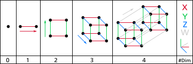
A drawing of the first four dimensions. On the left is zero dimensions (a point) and on the right is four dimensions (A tesseract). There is an axis and labels on the right and which level of dimensions it is on the bottom. The arrows alongside the shapes indicate the direction of extrusion.

Hypercube: n-dimensional analogue of a square (n = 2) and a cube n = 3). It is a closed, compact, convex figure whose 1-skeleton consists of groups of opposite parallel line segments aligned in each of the space's dimensions, perpendicular to each other and of the same length. A unit hypercube's longest diagonal in n dimensions is equal to ${\sqrt {n}}$.

Convex function: real-valued function is called convex if the line segment between any two points on the graph of the function lies above the graph between the two points. In simple terms, a convex function refers to a function whose graph is shaped like a cup $\cup$, while a concave function's graph is shaped like a cap $\cap$.

Saddle point (minimax point): point on the surface of the graph of a function where the slopes (derivatives) in orthogonal directions are all zero (a critical point), but which is not a local extremum of the function.

Group theory

Category:Group theory

Category:Coxeter groups

Group theory: studies the algebraic structures known as groups. The concept of a group is central to abstract algebra: other well-known algebraic structures, such as rings, fields, and vector spaces, can all be seen as groups endowed with additional operations and axioms. Groups recur throughout mathematics, and the methods of group theory have influenced many parts of algebra. Linear algebraic groups and Lie groups are two branches of group theory that have experienced advances and have become subject areas in their own right. Various physical systems, such as crystals and the hydrogen atom, may be modelled by symmetry groups. Thus group theory and the closely related representation theory have many important applications in physics, chemistry, and materials science. Group theory is also central to public key cryptography.

Coxeter group: abstract group that admits a formal description in terms of mirror symmetries.

Coxeter–Dynkin diagram (Coxeter diagram, Coxeter graph): graph with numerically labeled edges (called branches) representing the spatial relations between a collection of mirrors (or reflecting hyperplanes). Dynkin diagrams: closely related objects, which differ from Coxeter diagrams in two respects: firstly, branches labeled "4" or greater are directed, while Coxeter diagrams are undirected; secondly, Dynkin diagrams must satisfy an additional (crystallographic) restriction, namely that the only allowed branch labels are 2, 3, 4, and 6.

Symmetry group:

List of planar symmetry groups: what's the diff. with spherical symmetry groups? Plane vs sphere? Classes of discrete planar symmetry groups: 2 rosette groups (2D point groups) + 7 frieze groups (2D line groups) + 17 wallpaper groups (2D space groups)

List of spherical symmetry groups, spherical symmetry groups and point groups have the same notation. Are they qualitatively different? Or it's just the different way of putting graph theory (like binary vs. decimal, but still numbers)

Point group: group of geometric symmetries (isometries) that keep at least one point fixed; 1D, 2D, 3D, ..., 8D:

Point groups in two dimensions; point groups in 2D under crystallographic restriction theorem ⇒ wallpaper group (plane symmetry group or plane crystallographic group) [17]; frieze group

Point groups in three dimensions: 7 infinite families of axial (or prismatic groups), and 7 additional polyhedral (or Platonic groups) (Polyhedral group). Applying the crystallographic restriction theorem to these groups yields: 32 crystallographic point groups ((geometric) crystal classes)

Crystallographic point group (crystal class): tables: in Schoenflies [5*7=35, but 4 are forbidden and other 4 are the same as some others, so 35-4-4=27; add T, T_d, T_h, O and O_h [5]: 27+5=32], and in Hermann–Mauguin notations [32, table with empty (forbidden) spaces], and correspondence between different notations (crystal family & system, Hermann-Mauguin full & short symbols, Shubnikov, Schoenflies, orbifold, Coxeter, order) [32]

Notations for symmetry groups and point groups:

Coxeter notation (bracket notation): system of classifying symmetry groups, describing the angles between with fundamental reflections of a Coxeter group; uses a bracketed notation, with modifiers to indicate certain subgroups

Schoenflies notation (Schönflies notation): one of two conventions commonly used to describe Point groups; notation is used in spectroscopy (for molecular symmetry). Point group in the Schoenflies convention is completely adequate to describe the symmetry of a molecule; this is sufficient for spectroscopy. The Hermann–Maunguin notation is able to describe the space group of a crystal lattice, while the Schoenflies notation isn't. Thus the Hermann–Mauguin notation is used in crystallography.

Hermann–Mauguin notation (International notation (International Tables For Crystallography)): the other convention to commonly used to describe Point groups; used in crystallography (crystal symmetries in X-ray, neutron, electron, ...). Mirror plane (rotoinversion axis 2) is m, while the other rotoinversion axes are represented by the corresponding number with a macron, n — 1, 3, 4, 5, 6, 7, 8...

Orbifold notation (orbifold signature): system, invented by William Thurston (William Paul Thurston, of orbifold fame) and popularized by the mathematician John Conway, for representing types of symmetry groups in two-dimensional spaces of constant curvature. The advantage of the notation is that it describes these groups in a way which indicates many of the groups' properties: in particular, it describes the orbifold obtained by taking the quotient of Euclidean space by the group under consideration.

Fibrifold & fibrifold notation (in 3D): extension of orbifold notation for 3D space groups.

Schläfli symbol: notation of the form {p,q,r,...} that defines regular polytopes and tessellations (List of regular polytopes).

Wythoff symbol: first used by Coxeter, Longeut-Higgens and Miller in their enumeration of the uniform polyhedra.

Discrete mathematics

Category:Discrete mathematics

Category:Discrete geometry

Category:Packing problems

Kissing number: e.g. materials science, chem, phys - dense packing of atoms: only two possibilities in 3D: FCC (face-centered cubic) and HCP (hexagonal close-packed) [or a hybrid of both]

Mathematical analysis

Category:Mathematical analysis

Category:Asymptotic analysis

Category:Complex analysis

Category:Fields of mathematical analysis

Category:Functional analysis

Category:Operator theory

Category:Fixed points (mathematics)

Category:Fourier analysis

Category:Functions and mappings

Category:Types of functions

Category:Norms (mathematics)

Category:Normed spaces

Category:Banach spaces

Category:Hilbert spaces

Category:Numerical analysis

Stirling's approximation: approximation for factorials: $n!\sim {\sqrt {2\pi n}}\left({\frac {n}{e}}\right)^{n}$

Fixed point (mathematics) (fixpoint, invariant point): of a function is an element of the function's domain that is mapped to itself by the function. c is a fixed point of the function f(x) if and only if f(c) = c. This means f(f(...f(c)...)) = fⁿ(c) = c, an important terminating consideration when recursively computing f. A set of fixed points is sometimes called a fixed set. In graphical terms, a fixed point means the point (x, f(x)) is on the line y = x, or in other words the graph of f has a point in common with that line. Attractive fixed points; Generalization to partial orders: prefixpoint and postfixpoint.

Curse of dimensionality: various phenomena that arise when analyzing and organizing data in high-dimensional spaces (often with hundreds or thousands of dimensions) that do not occur in low-dimensional settings such as the three-dimensional physical space of everyday experience. The common theme of these problems is that when the dimensionality increases, the volume of the space increases so fast that the available data become sparse. This sparsity is problematic for any method that requires statistical significance. In order to obtain a statistically sound and reliable result, the amount of data needed to support the result often grows exponentially with the dimensionality.

Hilbert spaces: allow the methods of linear algebra and calculus to be generalized from (finite-dimensional) Euclidean vector spaces to spaces that may be infinite-dimensional. Hilbert spaces arise naturally and frequently in mathematics and physics, typically as function spaces. Formally, a Hilbert space is a vector space equipped with an inner product that defines a distance function for which the space is a complete metric space.

Fourier analysis

Category:Fourier analysis

Dirac delta function (δ function) is a generalized function or distribution introduced by the physicist Paul Dirac. It is used to model the density of an idealized point mass or point charge as a function equal to zero everywhere except for zero and whose integral over the entire real line is equal to one. As there is no function that has these properties, the computations made by the theoretical physicists appeared to mathematicians as nonsense until the introduction of distributions by Laurent Schwartz to formalize and validate the computations. As a distribution, the Dirac delta function is a linear functional that maps every function to its value at zero. The Kronecker delta function, which is usually defined on a discrete domain and takes values 0 and 1, is a discrete analog of the Dirac delta function. In engineering and signal processing, the delta function, also known as the unit impulse symbol, may be regarded through its Laplace transform, as coming from the boundary values of a complex analytic function of a complex variable. The formal rules obeyed by this function are part of the operational calculus, a standard tool kit of physics and engineering.

Discrete Fourier transform (DFT): FFT algorithms are so commonly employed to compute DFTs that the term "FFT" is often used to mean "DFT" in colloquial settings.

Relationship between the continuous Fourier transform and the discrete Fourier transform. Left column: A continuous function and its fourier transform. Center-left: If the function is periodically repeated, its fourier transform becomes zero except at discrete points. Center-right column: Likewise, if the function is discretized (by multiplying it by the Dirac comb), its fourier transform becomes periodic. Right column: If a function is both discrete and periodic, so is its Fourier transform. The right column corresponds mathematically to the discrete fourier transform.

Gibbs phenomenon: discovered by Henry Wilbraham (1848) and rediscovered by J. Willard Gibbs (1899), is the peculiar manner in which the Fourier series of a piecewise continuously differentiable periodic function behaves at a jump discontinuity. The nth partial sum of the Fourier series has large oscillations near the jump, which might increase the maximum of the partial sum above that of the function itself. The overshoot does not die out as n increases, but approaches a finite limit. This is one cause of ringing artifacts in signal processing.

Special functions

Category:Special functions

Category:Elementary special functions

Special functions: particular mathematical functions which have more or less established names and notations due to their importance in mathematical analysis, functional analysis, physics, or other applications.

Plot of the graphs of ${\tfrac {\sin(x)}{x}}$ (red) and ${\tfrac {\sin(\pi x)}{\pi x}}$ (blue) using cubic Bézier curves.

Sinc function

• in mathematics, the historical unnormalized sinc function is defined for x ≠ 0 by

$\operatorname {sinc} x={\frac {\sin x}{x}}.$

• In digital signal processing and information theory, the normalized sinc function is commonly defined for x ≠ 0 by

$\operatorname {sinc} x={\frac {\sin(\pi x)}{\pi x}}.$

Logit: function is the inverse of the sigmoidal "logistic" function or logistic transform used in mathematics, especially in statistics. When the function's variable represents a probability p, the logit function gives the log-odds, or the logarithm of the odds p/(1 − p). Comparison with probit: Closely related to the logit function (and logit model) are the probit function and probit model. The logit and probit are both sigmoid functions with a domain between 0 and 1, which makes them both quantile functions—i.e., inverses of the cumulative distribution function (CDF) of a probability distribution. In fact, the logit is the quantile function of the logistic distribution, while the probit is the quantile function of the normal distribution. As shown in the graph, the logit and probit functions are extremely similar, particularly when the probit function is scaled so that its slope at y=0 matches the slope of the logit. As a result, probit models are sometimes used in place of logit models because for certain applications (e.g., in Bayesian statistics) the implementation is easier.

Gamma function: extension of the factorial function, with its argument shifted down by 1, to real and complex numbers. $\Gamma (n)=(n-1)!$

Chaos theory, dynamical systems

Category:Dynamical systems {q.v. User:Kazkaskazkasako/Books/All#Dynamical systems}

Category:Bifurcation theory

Category:Chaos theory

Category:Chaotic maps

The xy-plane here represents to Re[c] and Re[i] plane, just as canonical Mandelbrot sets are considered. The z axis encodes the values that z[n] takes during its iteration. Thus, the areas unbounded (not in the Mandelbrot set) are mostly dark, and the areas bounded during iteration add up.

Logistic map: polynomial mapping (equivalently, recurrence relation) of degree 2, often cited as an archetypal example of how complex, chaotic behaviour can arise from very simple non-linear dynamical equations. The map was popularized in a seminal 1976 paper by the biologist Robert May, in part as a discrete-time demographic model analogous to the logistic equation first created by Pierre François Verhulst.

$\qquad x_{n+1}=rx_{n}(1-x_{n})$

where $x_{n}$ is a number between zero and one that represents the ratio of existing population to the maximum possible population. The values of interest for the parameter r are those in the interval (0, 4]. Behavior dependent on r; Chaos and the logistic map.

Bifurcation theory

Bifurcation diagram: shows the values visited or approached asymptotically (fixed points, periodic orbits, or chaotic attractors) of a system as a function of a bifurcation parameter in the system. It is usual to represent stable values with a solid line and unstable values with a dotted line, although often the unstable points are omitted.

Applied mathematics

Category:Applied mathematics

Category:Mathematical physics

{q.v. User:Kazkaskazkasako/Books/Physical sciences#Theoretical physics}

Mathematical proofs

Category:Mathematical proofs

Category:Proof without words

Proof without words (visual proof): proof of an identity or mathematical statement which can be demonstrated as self-evident by a diagram without any accompanying explanatory text. Such proofs can be considered more elegant than formal or mathematically rigorous due to their self-evident nature. When the diagram demonstrates a particular case of a general statement, to be a proof, it must be generalisable.

Geometric proof without words that max (a,b) > root mean square (RMS) or quadratic mean (QM) > arithmetic mean (AM) > geometric mean (GM) > harmonic mean (HM) > min (a,b) of two distinct positive numbers a and b

$max(a,b)$ > root mean square (RMS)/quadratic mean (QM) > arithmetic mean (AM) > geometric mean (GM) > harmonic mean (HM) > $min(a,b)$ of two positive numbers $a$ and $b$.