Talk:Cubic function/Archive 4

Needs clear algorithm

I'm writing software that needs to do a cubic solve. In Python, numpy.roots works great, but is slow for solving thousands of them in parallel, so I came here in search of the algorithm... but it isn't at all clear what the full algorithm is. Other web pages fail me too.

Am I just blind, or are none of the algorithms listed completely? In the "General formula of roots" section, it says if $-27a^{2}\Delta >0$, then the solutions are ___. But then it gives caveats and the version with Q and C, but that also has caveats. Is that Q and C version complete? If so, it doesn't read like an algorithm... —Ben FrantzDale (talk) 13:40, 11 October 2011 (UTC)

Do you really need a cubic solver whose output is thousands formulas with cubic and square roots inside? This seems incredible. I guess that you want numerical output. For this it is clearly better to use a root finding algorithm, because computing a numerical approximation of the roots of a cubic equation with a root finding algorithm is usually much faster than evaluating numerically the formula. In fact evaluating the formula implies to compute a square root, a cubic root and several other operations. Cubic root extraction is not really faster than a general root finding algorithm applied to a general cubic equation. D.Lazard (talk) 21:08, 12 October 2011 (UTC)

You may be right about performance. I had sort of assumed that since cubics can be solved in closed form, that it would be faster than an iterative approach. Still, the "algorithms" on the page aren't at all clear. I should be able to use the information on this page to find the roots of a cubic function, but attempts to follow the steps failed, usually in ambiguity. —Ben FrantzDale (talk) 13:08, 13 October 2011 (UTC)

I do not agree with you about the clarity of the "algorithms": The formula involving $C$ and $Q$ looks perfectly like an algorithm. It specifies the auxiliary functions (square and cubic roots). Its main difference with a well written algorithm is that the simple cases are at the end while a program is easier to read if the simple cases are at the beginning. Another difference with a well written algorithm is that in a program, names will be given to the expressions which appear several times, to avoid to compute them several times. For better readability, names have been given only to the quantities whose sign or equality to 0 have to be tested. I do not see any way to improve the algorithmic aspect of this page, while keeping a good readability, especially for beginners. Note that the first general formula is not useful from a logical point of view, and could thus be suppressed. But it has to appear, as it is the formula which is the most popular. D.Lazard (talk) 10:58, 14 October 2011 (UTC)

Some times ago I saw that sympy implement Cardano's formulas. However, I would have to consult the source again to find out if it is in any way stabilized. It is not to much effort to first implement the shift and then use the simple steps of the derivation.--LutzL (talk) 13:35, 13 October 2011 (UTC)

I must have been mistaken. I just re-tried coding the Q, C algorithm and it seems to work up to rounding error. For reference. This implementation solves many 4xn vectors at the same time (hence the lack of if/else and instead the use of masked arrays):

def solveCubicRoots(p):
    p = asarray(p)
    if p.ndim == 1:
        return solveCubicRoots(p[:,None])[:,0]
    p = cast[complex](p)
    a, b, c, d = p
    b2m3ac = b**2 - 3*a*c
    Q = sqrt((2*b**3 - 9*a*b*c+27*a**2*d)**2 - 4 * (b**2-3*a*c)**3)
    def CofQ(Q, m): 
        a, b, c, d = p[:,m]
        return (0.5*(Q+2*b**3-9*a*b*c+27*a**2*d))**(1./3.)

    result = zeros(p[:3].shape, dtype=complex)
    
    # Four cases: zero or not for Q and for b2m3ac:
    ZZ = logical_and(Q == 0, b2m3ac == 0)
    ZN = logical_and(Q == 0, b2m3ac != 0)
    NZ = logical_and(Q != 0, b2m3ac == 0)
    NN = logical_and(Q != 0, b2m3ac != 0)

    a, b, c, d = p[:,ZZ]
    result[:,ZZ] = -b/3*a
        
    a, b, c, d = p[:,ZN]
    result[:2,ZN] = (b*c - 9*a*d)/(2*(3*a*c-b**2))
    result[2,ZN] = (9*a**2*d-4*a*b*c+b**3)/(a*(3*a*c-b**2))
    
    QNZ = (Q != 0)
    C = CofQ(Q[QNZ], QNZ)
    mask = QNZ.copy()
    mask[QNZ] = logical_and(b2m3ac[QNZ] == 0, C == 0)
    C[mask] = CofQ(-Q[mask], mask)
    a, b, c, d = p[:,QNZ]
    i = complex(0,1)
    result[0,QNZ] = (-b - C - (b**2-3*a*c)/C)/(3*a)
    result[1,QNZ] = -b/(3*a) + C*(1+i*sqrt(3))/(6*a) + (1-i*sqrt(3))*(b**2-3*a*c)/(6*a*C)
    result[2,QNZ] = -b/(3*a) + C*(1-i*sqrt(3))/(6*a) + (1+i*sqrt(3))*(b**2-3*a*c)/(6*a*C)
    
    a, b, c, d = p[:,ZZ]
    result[:,ZZ] = -b/(3*a)

    return result

I may rephrase the description of this algorithm to make the description more imperative. —Ben FrantzDale (talk) 14:53, 17 October 2011 (UTC)

Anachronism?

In the history section, I read: Omar Khayyám (1048–1131) ... found a geometric solution which could be used to get a numerical answer by consulting trigonometric tables. I do not believe that, at that time, it was usual to use numerical tables to solve equations. In any case the assertion which could be used to get a numerical answer by consulting trigonometric tables is not sourced. On the other hand, the use of abaci to solve graphically numerical problem was very usual during the XVIe century and surely much before . Therefore I have edited this page, replacing which could be used ... by which could be used to get graphically a numerical answer. This seems less anachronistic. This has been reverted with the explanation that Hipparchus compiled trigonometric tables in the 1st century. OK, but this is not an indication that Omar Khayyám did use them. As I am unable to source my belief about graphical computation at that time, and I wish not to begin an edit war, I simply propose to remove the questionable assertion which could be used to get a numerical answer by consulting trigonometric tables. D.Lazard (talk) 18:54, 6 November 2011 (UTC)

I'm not taking sides here because I don't know the history. But I would mention that the article on Omar Khayyám simply says

He is the author of one of the most important treatises on algebra written before modern times, the Treatise on Demonstration of Problems of Algebra, which includes a geometric method for solving cubic equations by intersecting a hyperbola with a circle.[4]

No mention of trig. In fact, later on the article says

...on Khayyám's celebrated approach and method in geometric algebra and in particular in solving cubic equations. In that his solution is not a direct path to a numerical solution and in fact his solutions are not numbers but rather line segments.

That's a pretty specific assertion: his solutions are not numbers.

On the other hand, the article on trigonometry says

By the 10th century, Islamic mathematicians were using all six trigonometric functions, had tabulated their values, and were applying them to problems in spherical geometry. Duoduoduo (talk) 19:16, 6 November 2011 (UTC)

I have cn-tagged that statement. DVdm (talk) 11:15, 8 November 2011 (UTC)

Geometric interpretation of the roots

This section is a very good idea. However, as it is, without any figure, it is difficult to understand, even for an expert (I believe I am one). Even with figures, more explanation would be needed:

Section Three real roots: The geometric interpretation given in the caption of the figure at the top of the article should be recalled here. As given here, the geometric interpretation of Vieta's trigonometric formula appears to be simply an explanation of what a cosine and an arccosine are. Thus a figure is needed on which an equilateral triangle inscribed in a circle appears, whose edges project on the roots. A further explanation is needed, showing how the circle and the angle which has to be trisected may be graphically constructed.

Section In the Cartesian plane: Here also a figure is needed. Probably one should add a proof that this interpretation of the complex roots is correct, but this may be discussed. I have done an algebraic proof. A purely geometric proof would be much better if any.

Section In the complex plane: As written, the object of this section is not clear, as it consider the roots as given. Thus I would have began it as: "With one real and two complex roots, the three roots can be represented as points in the complex plane, as well as the two roots of the derivative. There is an interesting relationship between all these roots ... " One may add somewhere the fact that the roots of the derivative are real or complex depending if the summit angle of the triangle is smaller or larger than π/3.

D.Lazard (talk) 21:39, 15 November 2011 (UTC)

Thanks for the suggestions. I've incorporated the wording changes and additions you suggested in the section In the complex plane. As for the other sections, unfortunately I have zero skills in drawing figures. I'll see if I can get someone to draw the relevant figures, and then I'll need instructions on how to bring them into Wikipedia. Is it necessary to use a particular graphics package in order to get it into Wikipedia? Duoduoduo (talk) 22:30, 15 November 2011 (UTC)

I, also, have few skills in drawing figure. However, in Wikipedia:Images there is some information. I had a look on the available images by searching files: cubic equation, and I have found File:Omar Kayyám - Geometric solution to cubic equation.svg which contains this image 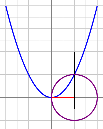and its explanation. This suggest to include another subsection, including this image and explaining this solution. D.Lazard (talk) 01:48, 16 November 2011 (UTC)

Done. Duoduoduo (talk) 17:32, 2 December 2011 (UTC)

This figure is quite misleading. It looks like the vertical line through the point of intersection of the circle and parabola also goes through the center of the circle. This makes the solution (the length of the red segment) in this case appear to be the radius of the circle. — Preceding unsigned comment added by 66.188.89.180 (talk) 13:44, 16 July 2012 (UTC)

Using trigonometric tables for solving a cubic equation in 11th centuries

As I have written before, such an assertion seems an anachronism. In fact, at these time, trigonometric values were not, as far as I know, computed numerically , but graphically (recall five centuries later, division was taught only in universities, in highest courses). It is thus highly improbable that Khayyam preferred to report in (graphical) the length obtained by the intersection of a circle and an ellipse than to simply measure this length.

JamesBWatson has just restored this controversial assertion, sourcing it by 3 references. The first one is a blog which reproduces textually the first one, without reference. It should thus be removed as non reliable, plagiarism and not useful. The third reference refers to [18] without any indication of what is [18]. Searching more, it appears that it is the version for printing of a page of MacTutor History of Mathematics and that [18] is the second reference. MacTutor is usually reliable but it may be wrong on some points. Thus I need to read this second reference to verify. It seems not to be on the net, but it seems to be in a library in my town. Thus I'll consult it tomorrow. For the moment I'll supress the first reference and tagging this citation. D.Lazard (talk) 18:35, 4 January 2012 (UTC)

For what it's worth, Derbyshire, John, Unknown Quantity: A Real and Imaginary History of Algebra, Plume, 2007, says on p. 54:

[Khayyam] posed and solved several problems involving cubic equations, though his solutions were always geometrical.

and then says on p. 55:

Khayyam took an indirect approach [to solving a particular cubic problem], ending up with a slightly different cubic, which he solved numerically via the intersection of two classic geometric curves.

This gets tantalizingly close, using the word numerically, but doesn't use the word trigonometrically. However, it seems to label as false the passage that I quoted in an earlier section on this talk page, from the Wiki page Omar Khayyám:

...on Khayyám's celebrated approach and method in geometric algebra and in particular in solving cubic equations. In that his solution is not a direct path to a numerical solution and in fact his solutions are not numbers but rather line segments.

Apparently he did somehow get numerical solutions from his geometric figures, contrary to that passage. Duoduoduo (talk) 21:20, 4 January 2012 (UTC)

This article has been edited by a user who is known to have misused sources to unduly promote certain views. See this edits. Examination of the sources used by this editor often reveals that the sources have been selectively interpreted or blatantly misrepresented, going beyond any reasonable interpretation of the authors' intent (see WP:Jagged 85 cleanup).

Tobby72 (talk) 15:43, 17 January 2012 (UTC)

Resolved

 – See note 8 in the article — D.Lazard (talk) 16:45, 17 January 2012 (UTC)

Suggestions

There are now six graphs plotted in the Cartesian (x&y) plane, but in corresponding text we have often f(x) instead y and always x even if unknown is t (4^th and 5^th graph).

(inserted comment) The graphs are not of depressed cubics, and are not intended to be, so they are in terms of x. But sometimes the text mentions the depressed case in terms of t, since that is sometimes easier to explain. So that is fine. Duoduoduo (talk) 10:19, 21 January 2012 (UTC)

Since we deal with polynomials of degree 3 it seems to me suitable to write $y=p_{3}(x).$

(inserted comment) f is a commonly used function name--no need to change it. Duoduoduo (talk) 10:19, 21 January 2012 (UTC)

In case of Depressed cubic the point of the inflection and of uneven Symmetry S(t=0,y=q) must be on y-axis which isn’t respected at fourth and fifth graph.

(inserted comment) Those graphs are of the general, not depressed, case. Duoduoduo (talk) 10:19, 21 January 2012 (UTC)

None of six graphs is presenting the cubic where either p > 0 or p = 0!

(inserted comment) p is a parameter of the depressed case, which none of the graphs show. However, all cubics are linear transformations of the depressed case, in which p=0 or p>0 is a sufficient (but not necessary) condition for one real root. The next-to-last graph shows the case of a non-depressed cubic with one real root. Duoduoduo (talk) 10:19, 21 January 2012 (UTC)

The chapter-name Derivative could be set in plural Derivatives

(inserted comment) There is only one derivative: f ′(x) = 3ax² + 2bx + c. Duoduoduo (talk) 10:19, 21 January 2012 (UTC)

and extended by:

$p''_{3}(x)=6ax+2b=0{\text{ for }}x=s={\frac {-b}{3a}}$

which is necessary condition and

$p_{3}^{(3)}(x)=6a\not =0$

which, since it doesn’t change a sign for any x, is sufficient condition for S(s = 1,q = 286) to be point of the inflection, of uneven Symmetry as well (see Wikipedia article on Inflection point where from the graph is overtaken and where negative sign before 400 at lower turning point is also missing).

The warning to y vs. x aspect ratio should be at least mentioned (y : x = 49 :1) but, even if so, the geometry is lost: a circle will be squeezed to an ellipse, a normal line will not seem perpendicular to tangency etc. This inconveniency can be avoided by means of the routine applied at "Trigonometric (and hyperbolic) method" where monic depressed cubic equation is, in fact, converted into its canonical form.

Graphical Function Explorer (GFE) is an easily handled but very suitable graphing tool where the variables a, b, c, d and unknown x (lower case) are default. Therefore a_{0; 1; 2; 3} is selected for variables as well as X (upper case) as unknown of cubic general form.

${\frac {p_{3}(X)}{a_{3}}}={\frac {a_{3}X^{3}+a_{2}X^{2}+a_{1}X+a_{0}}{a_{3}}}=(X-s)^{3}+p(X-s)+q=0{\big |}*{\frac {4}{R^{3}}},s={\frac {-a_{2}}{3a_{3}}},R=-{\frac {2q}{|q|}}{\sqrt {\frac {|p|}{3}}}\Rightarrow$

$4\left({\frac {X-s}{R}}\right)^{3}+{\frac {3p}{|p|}}\left({\frac {X-s}{R}}\right)=4x^{3}+{\frac {3p}{|p|}}x={\frac {4q}{R^{3}}}\geq 0{\text{ and }}X=s+Rx=s-{\frac {2q}{|q|}}{\sqrt {\frac {|p|}{3}}}x.$

This conversion is applied below to three characteristic examples composed of the variables being abscise (s), slope (p) and ordinate (q) of the inflection point:

$s={\frac {-a_{2}}{3a_{3}}}=1,{\text{ }}p={\frac {p'_{3}(s)}{a_{3}}}=\mp 3*7^{2}{\text{ and }}q={\frac {p_{3}(s)}{a_{3}}}=2*143;-2*872;-2*74.$

$X^{3}-3X^{2}-144X+432=(X-1)^{3}-3*7^{2}(X-1)+2*143=0{\big |}*{\frac {-4}{14^{3}}}{\text{ which can be bisected into:}}$ $4\left({\frac {X-1}{-2*7}}\right)^{3}-3\left({\frac {X-1}{-2*7}}\right)=4x^{3}-3x=f(x)=g(x)={\frac {143}{7^{3}}}\approx 0.4169<1{\text{ and }}p<0.$

$X^{3}-3X^{2}-144X-1598=(X-1)^{3}-3*7^{2}(X-1)-2*872=0{\big |}*{\frac {4}{14^{3}}}{\text{ which can be bisected into:}}$ $4\left({\frac {X-1}{2*7}}\right)^{3}-3\left({\frac {X-1}{2*7}}\right)=4x^{3}-3x=f(x)=h(x)={\frac {872}{7^{3}}}\approx 1.7055>1{\text{ and }}p<0.$

$X^{3}-3X^{2}+152X-300=(X-1)^{3}+3*7^{2}(X-1)-2*74=0{\big |}*{\frac {4}{14^{3}}}{\text{ which can be bisected into:}}$ $4\left({\frac {X-1}{2*7}}\right)^{3}+3\left({\frac {X-1}{2*7}}\right)=4x^{3}+3x=f(x)=h(x)={\frac {74}{7^{3}}}\approx 0,21574>0{\text{ and }}p>0.$

Opening

http://www.mathopenref.com/graphfunctions.html?fx=(3*b%5e2+1)*x%5e3+3*b*x%20&gx=a*(3*((c/d)%5e2+b)*(x-c/d)+872/7%5e3)+(1-a)*143/7%5e3&hx=a*6*((c/d)%5e2+b)*(x-c/d)+872/7%5e3&xh=2&yl=-1.5&ah=1&a=0&bh=1&bl=-1&b=-1&ch=99&c=16&dh=99&dl=1&d=14&cr=t&cx=1.14286

we get an image enabling graphical resolving of all cubic equation types.

For initial setting (a = 0, b = –1, c = 16 and d = 14) black horizontal straight line g(x) intercepts f(x) at three points but red one h(x) at only one. The abscises of these points are real roots of canonical cubic form for first and second example where p < 0:

$g(x)={\frac {143}{7^{3}}}<1{\text{ intercepts }}f(x)=4x^{3}-3x{\text{ at the points determining 3 real roots:}}$

${\frac {143}{7^{3}}}=f\left(-0.1429\approx -{\frac {2}{14}}\right)=f\left(-0.7857\approx -{\frac {11}{14}}\right)=f\left(0.9286\approx {\frac {13}{14}}\right)$

giving after back-conversion: $X_{k}=1-{\frac {14*q}{|q|}}*x_{k}=3;\pm 12.$

$h(x)={\frac {872}{7^{3}}}\approx 2.5423>1{\text{ intercepts }}f(x)=4x^{3}-3x{\text{ at R where }}x_{R}\approx 1.14286={\frac {16}{14}}={\frac {c}{d}}$ giving after back-conversion $X_{R}=1-{\frac {14*q}{|q|}}*x_{R}=1+16=17.$

For a = 1 g(x) becomes tangency of f(x) at point H intercepting f(x) at point R but h(x) intercepts f(x) at three points R, A and B determining real (Re) and imaginary (Im) part of conjugate roots as presented at chapter 3.8.2.1 of the article.

$Re(x_{1;2})=x_{H}=-{\frac {x_{R}}{2}}=-{\frac {4}{7}}\approx -0.5714,x_{A}\approx -0.0922,Im(x_{1;2})=x_{A}-x_{H}={\frac {\sqrt {45}}{14}}\approx 0,4792.$

Setting b = +1 and replacing 872 by 74 in the boxes for f(x) and h(x) GFE returns

$h(x)={\frac {74}{7^{3}}}\approx 0.2157{\text{ intercepts }}f(x)=4x^{3}+3x{\text{ at R where }}x_{R}\approx 0.0714={\frac {1}{14}}={\frac {c}{d}}$

giving after back-conversion $X_{R}=1-{\frac {14*q}{|q|}}*x_{R}=1+1=2.$

$Re(x_{1;2})=x_{H}=-{\frac {x_{R}}{2}}=-{\frac {1}{28}}\approx 0.0357,x_{A}\approx -0.8325,Im(x_{1;2})=x_{A}-x_{H}={\frac {\sqrt {591}}{28}}\approx 0,8682.$

http://www.mathopenref.com/cubicexplorer.html is already included as External link. Perhaps the author could update it as suggested above.

Stap217.197.142.0 (talk) 05:42, 21 January 2012 (UTC)

Everything looks fine to me as is, and I think putting in the extended information that you suggest would make an already very long article too long. Also, see my inserted comments above. Duoduoduo (talk) 10:19, 21 January 2012 (UTC)

On the contrary, my intention was to show how this long article can be shortened rooming three images into the slightly expanded image from chapter “Derivative” the textual part of which would be completed with few additional lines as D. Lazard formulated below. You claim above that in graphs 3 and 4 are not depressed cubic but in second line of joined text is $t^{3}+pt+q$ along with its roots in next line. Moreover there is comment at File history authorized by Duoduoduo: ({{Information |Description = For the depressed cubic $t^{3}+pt+q=0$ with three real roots, the roots form an equilateral triangle with vertices A, B, and C in the circle. The angle... It confuses me. The easiest way to avoid this incoherence is to rename abscise x to t setting f(t)-axis at the inflection point and center of the circle. Stap217.197.142.0 (talk) 18:29, 24 January 2012 (UTC)

The summary box of the graph file was incorrect -- I should have been more careful in writing it, and I have now corrected it. Thanks for pointing it out! However, I don't have the graphics skills to redraw the graph for the shifted depressed case, and anyway I think there's value in showing graphically that the statement in the text that a trig approach is possible remains true for the non-depressed case. Duoduoduo (talk) 21:32, 24 January 2012 (UTC)

Shape of the displayed cubics: The remark of the IP user is worthwhile, even if it is not well expressed: All the displayed cubics have the same shape: two real roots for the derivative and a positive third derivative (leading coefficient). It would be useful to display all the four different possible shapes (in fact 6 if one counts the cases of a double root of the derivative). D.Lazard (talk) 11:16, 21 January 2012 (UTC)

Section Derivative: I do not agree with the IP users on the change of name, but I agree on the expansion of the section: That is to introduce the successive derivatives and to explain that the root of the second derivative gives the inflexion point and that, up to a factor of 6, the 3d derivative is the leading coefficient, and that its sign says if the infinite branches are increasing or decreasing. D.Lazard (talk) 11:16, 21 January 2012 (UTC)

Setting unary operator b successively to –1, 0, +1 GFE returns three shapes of f(x) where the infinite branches are increasing. Entering minus at the beginning of f-box we get remaining three shapes where the infinite branches are decreasing. Stap217.197.142.0 (talk) 18:29, 24 January 2012 (UTC)

Note — See multiple talk page abuse warnings to IP (aka STAP) at User talk:188.127.120.154. - DVdm (talk) 12:22, 21 January 2012 (UTC)