
Discrete dipole approximation

Discrete dipole approximation (DDA), also known as coupled dipole approximation,[1] is a method for computing scattering of radiation by particles of arbitrary shape and by periodic structures. Given a target of arbitrary geometry, one seeks to calculate its scattering and absorption properties by an approximation of the continuum target by a finite array of small polarizable dipoles. This technique is used in a variety of applications including nanophotonics, radar scattering, aerosol physics and astrophysics.
Basic concepts[edit]
The basic idea of the DDA was introduced in 1964 by DeVoe[2] who applied it to study the optical properties of molecular aggregates; retardation effects were not included, so DeVoe's treatment was limited to aggregates that were small compared with the wavelength. The DDA, including retardation effects, was proposed in 1973 by Purcell and Pennypacker[3] who used it to study interstellar dust grains. Simply stated, the DDA is an approximation of the continuum target by a finite array of polarizable points. The points acquire dipole moments in response to the local electric field. The dipoles interact with one another via their electric fields, so the DDA is also sometimes referred to as the coupled dipole approximation.[1][4]
Nature provides the physical inspiration for the DDA - in 1909 Lorentz[5] showed that the dielectric properties of a substance could be directly related to the polarizabilities of the individual atoms of which it was composed, with a particularly simple and exact relationship, the Clausius-Mossotti relation (or Lorentz-Lorenz), when the atoms are located on a cubical lattice. We may expect that, just as a continuum representation of a solid is appropriate on length scales that are large compared with the interatomic spacing, an array of polarizable points can accurately approximate the response of a continuum target on length scales that are large compared with the interdipole separation.
For a finite array of point dipoles the scattering problem may be solved exactly, so the only approximation that is present in the DDA is the replacement of the continuum target by an array of N-point dipoles. The replacement requires specification of both the geometry (location of the dipoles) and the dipole polarizabilities. For monochromatic incident waves the self-consistent solution for the oscillating dipole moments may be found; from these the absorption and scattering cross sections are computed. If DDA solutions are obtained for two independent polarizations of the incident wave, then the complete amplitude scattering matrix can be determined. Alternatively, the DDA can be derived from volume integral equation for the electric field.[6] This highlights that the approximation of point dipoles is equivalent to that of discretizing the integral equation, and thus decreases with decreasing dipole size.
With the recognition that the polarizabilities may be tensors, the DDA can readily be applied to anisotropic materials. The extension of the DDA to treat materials with nonzero magnetic susceptibility is also straightforward, although for most applications magnetic effects are negligible.
There are several reviews of DDA method. [7][6][8][9]
Extensions[edit]
The method was improved by Draine, Flatau, and Goodman, who applied the fast Fourier transform to solve fast convolution problems arising in the discrete dipole approximation (DDA). This allowed for the calculation of scattering by large targets. They distributed an open-source code DDSCAT.[7][10] There are now several DDA implementations,[6] extensions to periodic targets,[11] and particles placed on or near a plane substrate.[12][13] Comparisons with exact techniques have also been published.[14] Other aspects, such as the validity criteria of the discrete dipole approximation, were published.[15] The DDA was also extended to employ rectangular or cuboid dipoles,[16] which are more efficient for highly oblate or prolate particles.
Fast Fourier Transform for fast convolution calculations[edit]
The Fast Fourier Transform (FFT) method was introduced in 1991 by Goodman, Draine, and Flatau[17] for the discrete dipole approximation. They utilized a 3D FFT GPFA written by Clive Temperton. The interaction matrix was extended to twice its original size to incorporate negative lags by mirroring and reversing the interaction matrix. Several variants have been developed since then. Barrowes, Teixeira, and Kong[18] in 2001 developed a code that uses block reordering, zero padding, and a reconstruction algorithm, claiming minimal memory usage. McDonald, Golden, and Jennings[19] in 2009 used a 1D FFT code and extended the interaction matrix in the x, y, and z directions of the FFT calculations, suggesting memory savings due to this approach. This variant was also implemented in the MATLAB 2021 code by Shabaninezhad and Ramakrishna[20]. Other techniques to accelerate convolutions have been suggested in a general context[21][22] along with faster evaluations of Fast Fourier Transforms arising in DDA problem solvers.
Conjugate gradient iteration schemes and preconditioning[edit]
Some of the early calculations of the polarization vector were based on direct inversion[3] and the implementation of the conjugate gradient method by Petravic and Kuo-Petravic.[23] Subsequently, many other conjugate gradient methods have been tested.[24] Advances in the preconditioning of linear systems of equations arising in the DDA setup have also been reported.[25]
Discrete dipole approximation codes[edit]
Most of the codes apply to arbitrary-shaped inhomogeneous nonmagnetic particles and particle systems in free space or homogeneous dielectric host medium. The calculated quantities typically include the Mueller matrices, integral cross-sections (extinction, absorption, and scattering), internal fields and angle-resolved scattered fields (phase function). There are some published comparisons of existing DDA codes.[14]
General-purpose open-source DDA codes[edit]
These codes typically use regular grids (cubical or rectangular cuboid), conjugate gradient method to solve large system of linear equations, and FFT-acceleration of the matrix-vector products which uses convolution theorem. Complexity of this approach is almost linear in number of dipoles for both time and memory.[6]
| Name | Authors | References | Language | Updated | Features |
|---|---|---|---|---|---|
| DDSCAT | Draine and Flatau | [7] | Fortran | 2019 (v. 7.3.3) | Can also handle periodic particles and efficiently calculate near fields. Uses OpenMP acceleration. |
| DDscat.C++ | Choliy | [26] | C++ | 2017 (v. 7.3.1) | Version of DDSCAT translated to C++ with some further improvements. |
| ADDA | Yurkin, Hoekstra, and contributors | [27][28] | C | 2020 (v. 1.4.0) | Implements fast and rigorous consideration of a plane substrate, and allows rectangular-cuboid voxels for highly oblate or prolate particles. Can also calculate emission (decay-rate) enhancement of point emitters. Near-fields calculation is not very efficient. Uses Message Passing Interface (MPI) parallelization and can run on GPU (OpenCL). |
| OpenDDA | McDonald | [19][29] | C | 2009 (v. 0.4.1) | Uses both OpenMP and MPI parallelization. Focuses on computational efficiency. |
| DDA-GPU | Kieß | [30] | C++ | 2016 | Runs on GPU (OpenCL). Algorithms are partly based on ADDA. |
| VIE-FFT | Sha | [31] | C/C++ | 2019 | Also calculates near fields and material absorption. Named differently, but the algorithms are very similar to the ones used in the mainstream DDA. |
| VoxScatter | Groth, Polimeridis, and White | [32] | Matlab | 2019 | Uses circulant preconditioner for accelerating iterative solvers |
| IF-DDA | Chaumet, Sentenac, and Sentenac | [33] | Fortran, GUI in C++ with Qt | 2021 (v. 0.9.19) | Idiot-friendly DDA. Uses OpenMP and HDF5. Has a separate version (IF-DDAM) for multi-layered substrate. |
| MPDDA | Shabaninezhad, Awan, and Ramakrishna | [20] | Matlab | 2021 (v. 1.0) | Runs on GPU (using Matlab capabilities) |
Specialized DDA codes[edit]
These list include codes that do not qualify for the previous section. The reasons may include the following: source code is not available, FFT acceleration is absent or reduced, the code focuses on specific applications not allowing easy calculation of standard scattering quantities.
| Name | Authors | References | Language | Updated | Features | |
|---|---|---|---|---|---|---|
| DDSURF, DDSUB, DDFILM | Schmehl, Nebeker, and Zhang | [12][34][35] | Fortran | 2008 | Rigorous handling of semi-infinite substrate and finite films (with arbitrary particle placement), but only 2D FFT acceleration is used. | |
| DDMM | Mackowski | [36] | Fortran | 2002 | Calculates T-matrix, which can then be used to efficiently calculate orientation-averaged scattering properties. | |
| CDA | McMahon | [37] | Matlab | 2006 | ||
| DDA-SI | Loke | [38] | Matlab | 2014 (v. 0.2) | Rigorous handling of substrate, but no FFT acceleration is used. | |
| PyDDA | Dmitriev | Python | 2015 | Reimplementation of DDA-SI | ||
| e-DDA | Vaschillo and Bigelow | [39] | Fortran | 2019 (v. 2.0) | Simulates electron-energy loss spectroscopy and cathodoluminescence. Built upon DDSCAT 7.1. | |
| DDEELS | Geuquet, Guillaume and Henrard | [40] | Fortran | 2013 (v. 2.1) | Simulates electron-energy loss spectroscopy and cathodoluminescence. Handles substrate through image approximation, but no FFT acceleration is used. | |
| T-DDA | Edalatpour | [41] | Fortran | 2015 | Simulates near-field radiative heat transfer. The computational bottleneck is direct matrix inversion (no FFT acceleration is used). Uses OpenMP and MPI parallelization. | |
| CDDA | Rosales, Albella, González, Gutiérrez, and Moreno | [42] | 2021 | Applies to chiral systems (solves coupled equations for electric and magnetic fields) | ||
| PyDScat | Yibin Jiang, Abhishek Sharma and Leroy Cronin | [43] | Python | 2023 | Simulates nanostructures undergoing structural transformation with GPU acceleration. |
Gallery of shapes[edit]
-
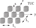 Scattering by periodic structures such as slabs, gratings, of periodic cubes placed on a surface, can be solved in the discrete dipole approximation.
 -
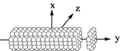 Scattering by infinite object (such as cylinder) can be solved in the discrete dipole approximation.


See also[edit]
- Computational electromagnetics
- Mie theory
- Finite-difference time-domain method
- Method of moments (electromagnetics)
References[edit]
- ^ a b Singham, Shermila B.; Salzman, Gary C. (1986). "Evaluation of the scattering matrix of an arbitrary particle using the coupled dipole approximation". J. Chem. Phys. 84 (5). AIP Publishing: 2658–2667. Bibcode:1986JChPh..84.2658S. doi:10.1063/1.450338.
- ^ DeVoe, Howard (1964-07-15). "Optical Properties of Molecular Aggregates. I. Classical Model of Electronic Absorption and Refraction". J. Chem. Phys. 41 (2). AIP Publishing: 393–400. Bibcode:1964JChPh..41..393D. doi:10.1063/1.1725879.
- ^ a b E. M. Purcell; C. R. Pennypacker (1973). "Scattering and absorption of light by nonspherical dielectric grains". Astrophys. J. 186: 705. Bibcode:1973ApJ...186..705P. doi:10.1086/152538.
- ^ Singham, Shermila Brito; Bohren, Craig F. (1987-01-01). "Light scattering by an arbitrary particle: a physical reformulation of the coupled dipole method". Opt. Lett. 12 (1). The Optical Society: 10–12. Bibcode:1987OptL...12...10S. doi:10.1364/ol.12.000010. PMID 19738776.
- ^ H. A. Lorentz, Theory of Electrons (Teubner, Leipzig, 1909)
- ^ a b c d M. A. Yurkin; A. G. Hoekstra (2007). "The discrete dipole approximation: an overview and recent developments" (PDF). J. Quant. Spectrosc. Radiat. Transfer. 106 (1–3): 558–589. arXiv:0704.0038. Bibcode:2007JQSRT.106..558Y. doi:10.1016/j.jqsrt.2007.01.034. S2CID 119572857.
- ^ a b c Draine, B.T.; P.J. Flatau (1994). "Discrete dipole approximation for scattering calculations". J. Opt. Soc. Am. A. 11 (4): 1491–1499. Bibcode:1994JOSAA..11.1491D. doi:10.1364/JOSAA.11.001491.
- ^ Yurkin, Maxim A. (2023). "Discrete Dipole Approximation". Light, Plasmonics and Particles. Elsevier. pp. 167–198.
- ^ Chaumet, Patrick Christian (2022). "The discrete dipole approximation: A review". Mathematics. 10 (17). MDPI: 3049. doi:10.3390/math10173049.
- ^ B. T. Draine; P. J. Flatau (2008). "The discrete dipole approximation for periodic targets: theory and tests". J. Opt. Soc. Am. A. 25 (11): 2693–3303. arXiv:0809.0338. Bibcode:2008JOSAA..25.2693D. doi:10.1364/JOSAA.25.002693. PMID 18978846. S2CID 15747060.
- ^ Chaumet, Patrick C.; Rahmani, Adel; Bryant, Garnett W. (2003-04-02). "Generalization of the coupled dipole method to periodic structures". Phys. Rev. B. 67 (16). American Physical Society (APS): 165404. arXiv:physics/0305051. Bibcode:2003PhRvB..67p5404C. doi:10.1103/physrevb.67.165404. S2CID 26726283.
- ^ a b Schmehl, Roland; Nebeker, Brent M.; Hirleman, E. Dan (1997-11-01). "Discrete-dipole approximation for scattering by features on surfaces by means of a two-dimensional fast Fourier transform technique". J. Opt. Soc. Am. A. 14 (11). The Optical Society: 3026–3036. Bibcode:1997JOSAA..14.3026S. doi:10.1364/josaa.14.003026.
- ^ M. A. Yurkin; M. Huntemann (2015). "Rigorous and fast discrete dipole approximation for particles near a plane interface" (PDF). The Journal of Physical Chemistry C. 119 (52): 29088–29094. doi:10.1021/acs.jpcc.5b09271.
- ^ a b Penttilä, Antti; Zubko, Evgenij; Lumme, Kari; Muinonen, Karri; Yurkin, Maxim A.; et al. (2007). "Comparison between discrete dipole implementations and exact techniques". J. Quant. Spectrosc. Radiat. Transfer. 106 (1–3). Elsevier BV: 417–436. Bibcode:2007JQSRT.106..417P. doi:10.1016/j.jqsrt.2007.01.026.
- ^ Zubko, Evgenij; Petrov, Dmitry; Grynko, Yevgen; Shkuratov, Yuriy; Okamoto, Hajime; et al. (2010-03-04). "Validity criteria of the discrete dipole approximation". Appl. Opt. 49 (8). The Optical Society: 1267–1279. Bibcode:2010ApOpt..49.1267Z. doi:10.1364/ao.49.001267. hdl:2115/50065. PMID 20220882.
- ^ D. A. Smunev; P. C. Chaumet; M. A. Yurkin (2015). "Rectangular dipoles in the discrete dipole approximation" (PDF). J. Quant. Spectrosc. Radiat. Transfer. 156: 67–79. Bibcode:2015JQSRT.156...67S. doi:10.1016/j.jqsrt.2015.01.019.
- ^ Goodman, John J.; Draine, Bruce T.; Flatau, Piotr J. (1991). "Application of fast-Fourier-transform techniques to the discrete-dipole approximation". Optics Letters. 16 (15). Optica Publishing Group: 1198–1200.
- ^ Barrowes, B. E.; Teixeira, F. L.; Kong, J. A. (2001). "Fast algorithm for matrix–vector multiply of asymmetric multilevel block‐Toeplitz matrices in 3‐D scattering". Microwave and Optical Technology Letters. 31 (1): 28–32.
- ^ a b J. McDonald; A. Golden; G. Jennings (2009). "OpenDDA: a novel high-performance computational framework for the discrete dipole approximation". Int. J. High Perf. Comp. Appl. 23 (1): 42–61. arXiv:0908.0863. Bibcode:2009arXiv0908.0863M. doi:10.1177/1094342008097914. S2CID 10285783.
- ^ a b M. Shabaninezhad; M. G. Awan; G. Ramakrishna (2021). "MATLAB package for discrete dipole approximation by graphics processing unit: Fast Fourier Transform and Biconjugate Gradient". J. Quant. Spectrosc. Radiat. Transfer. 262: 107501. Bibcode:2021JQSRT.26207501S. doi:10.1016/j.jqsrt.2020.107501. S2CID 233839571.
- ^ Fu, Daniel Y; Kumbong, Hermann; Nguyen, Eric; Ré, Christopher (2023). "FlashFFTConv: Efficient Convolutions for Long Sequences with Tensor Cores". arXiv:2311.05908 [cs.LG].
- ^ Bowman, John C.; Roberts, Malcolm (2011). "Efficient dealiased convolutions without padding". SIAM Journal on Scientific Computing. 33 (1). SIAM: 386–406. arXiv:1008.1366. Bibcode:2011SJSC...33..386B. doi:10.1137/100787933.
- ^ Petravic, M.; Kuo-Petravic, G. (1979). "An ILUCG algorithm which minimizes in the euclidean norm". Journal of Computational Physics. 32 (2): 263–269.
- ^ Chaumet, Patrick C. (2024). "A comparative study of efficient iterative solvers for the discrete dipole approximation". Journal of Quantitative Spectroscopy and Radiative Transfer. 312. Elsevier. Bibcode:2024JQSRT.31208816C. doi:10.1016/j.jqsrt.2023.108816. S2CID 264805146.
- ^ Chaumet, Patrick C.; Maire, Guillaume; Sentenac, Anne (2023). "Accelerating the discrete dipole approximation by initializing with a scalar solution and using a circulant preconditioning". Journal of Quantitative Spectroscopy and Radiative Transfer. 298. Elsevier. Bibcode:2023JQSRT.29808505C. doi:10.1016/j.jqsrt.2023.108505.
- ^ V. Y. Choliy (2013). "The discrete dipole approximation code DDscat.C++: features, limitations and plans". Adv. Astron. Space Phys. 3: 66–70. Bibcode:2013AASP....3...66C.
- ^ M. A. Yurkin; V. P. Maltsev; A. G. Hoekstra (2007). "The discrete dipole approximation for simulation of light scattering by particles much larger than the wavelength" (PDF). J. Quant. Spectrosc. Radiat. Transfer. 106 (1–3): 546–557. arXiv:0704.0037. Bibcode:2007JQSRT.106..546Y. doi:10.1016/j.jqsrt.2007.01.033. S2CID 119574693.
- ^ M. A. Yurkin; A. G. Hoekstra (2011). "The discrete-dipole-approximation code ADDA: capabilities and known limitations" (PDF). J. Quant. Spectrosc. Radiat. Transfer. 112 (13): 2234–2247. Bibcode:2011JQSRT.112.2234Y. doi:10.1016/j.jqsrt.2011.01.031.
- ^ J. McDonald (2007). OpenDDA - a novel high-performance computational framework for the discrete dipole approximation (PDF) (PhD). Galway: National University of Ireland.
- ^ M. Zimmermann; A. Tausendfreund; S. Patzelt; G. Goch; S. Kieß; M. Z. Shaikh; M. Gregoire; S. Simon (2012). "In-process measuring procedure for sub-100 nm structures". J. Laser Appl. 24 (4): 042010. Bibcode:2012JLasA..24d2010Z. doi:10.2351/1.4719936.
- ^ W. E. I. Sha; W. C. H. Choy; Y. P. Chen; W. C. Chew (2011). "Optical design of organic solar cell with hybrid plasmonic system". Opt. Express. 19 (17): 15908–15918. Bibcode:2011OExpr..1915908S. doi:10.1364/OE.19.015908. PMID 21934954.
- ^ S. P. Groth; A.G. Polimeridis; J.K. White (2020). "Accelerating the discrete dipole approximation via circulant preconditioning". J. Quant. Spectrosc. Radiat. Transfer. 240: 106689. Bibcode:2020JQSRT.24006689G. doi:10.1016/j.jqsrt.2019.106689. S2CID 209969404.
- ^ P. C. Chaumet; D. Sentenac; G. Maire; T. Zhang; A. Sentenac (2021). "IFDDA, an easy-to-use code for simulating the field scattered by 3D inhomogeneous objects in a stratified medium: tutorial". J. Opt. Soc. Am. A. 38 (12): 1841–1852. Bibcode:2021JOSAA..38.1841C. doi:10.1364/JOSAA.432685.
- ^ B. M. Nebeker (1998). Modeling of light scattering from features above and below surfaces using the discrete-dipole approximation (PhD). Tempe, AZ, USA: Arizona State University.
- ^ E. Bae; H. Zhang; E. D. Hirleman (2008). "Application of the discrete dipole approximation for dipoles embedded in film". J. Opt. Soc. Am. A. 25 (7): 1728–1736. Bibcode:2008JOSAA..25.1728B. doi:10.1364/JOSAA.25.001728. PMID 18594631.
- ^ D. W. Mackowski (2002). "Discrete dipole moment method for calculation of the T matrix for nonspherical particles". J. Opt. Soc. Am. A. 19 (5): 881–893. Bibcode:2002JOSAA..19..881M. doi:10.1364/JOSAA.19.000881. PMID 11999964.
- ^ M. D. McMahon (2006). Effects of geometrical order on the linear and nonlinear optical properties of metal nanoparticles (PDF) (PhD). Nashville, TN, USA: Vanderbilt University.
- ^ V. L. Y. Loke; P. M. Mengüç; Timo A. Nieminen (2011). "Discrete dipole approximation with surface interaction: Computational toolbox for MATLAB". J. Quant. Spectrosc. Radiat. Transfer. 112 (11): 1711–1725. Bibcode:2011JQSRT.112.1711L. doi:10.1016/j.jqsrt.2011.03.012.
- ^ N. W. Bigelow; A. Vaschillo; V. Iberi; J. P. Camden; D. J. Masiello (2012). "Characterization of the electron- and photon-driven plasmonic excitations of metal nanorods". ACS Nano. 6 (8): 7497–7504. doi:10.1021/nn302980u. PMID 22849410.
- ^ N. Geuquet; L. Henrard (2010). "EELS and optical response of a noble metal nanoparticle in the frame of a discrete dipole approximation". Ultramicroscopy. 110 (8): 1075–1080. doi:10.1016/j.ultramic.2010.01.013.
- ^ S. Edalatpour; M. Čuma; T. Trueax; R. Backman; M. Francoeur (2015). "Convergence analysis of the thermal discrete dipole approximation". Phys. Rev. E. 91 (6): 063307. arXiv:1502.02186. Bibcode:2015PhRvE..91f3307E. doi:10.1103/PhysRevE.91.063307. PMID 26172822. S2CID 21556373.
- ^ S. A. Rosales; P. Albella; F. González; Y. Gutierrez; F. Moreno (2021). "CDDA: extension and analysis of the discrete dipole approximation for chiral systems". Opt. Express. 29 (19): 30020–30034. Bibcode:2021OExpr..2930020R. doi:10.1364/OE.434061. hdl:10902/24774. PMID 34614734.
- ^ Jiang, Yibin; Sharma, Abhishek; Cronin, Leroy (2023). "An Accelerated Method for Investigating Spectral Properties of Dynamically Evolving Nanostructures". The Journal of Physical Chemistry Letters. 14 (16): 3929–3938. doi:10.1021/acs.jpclett.3c00395. PMC 10150391. PMID 37078273.